12.1 Introduction to R Markdown
R Markdown is an interactive and dynamic file format in R. An R Markdown file can be transformed into a document of many different types, including HTML, PDF, and Word.
12.1.1 Create a new R Markdown document
To create an R Markdown document, you can click the + button on the R Studio menu, then select R Markdown.
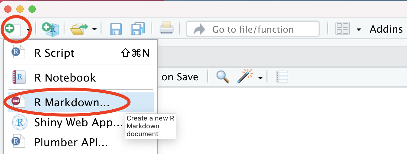
Figure 12.1: create a new R Markdown document (I)
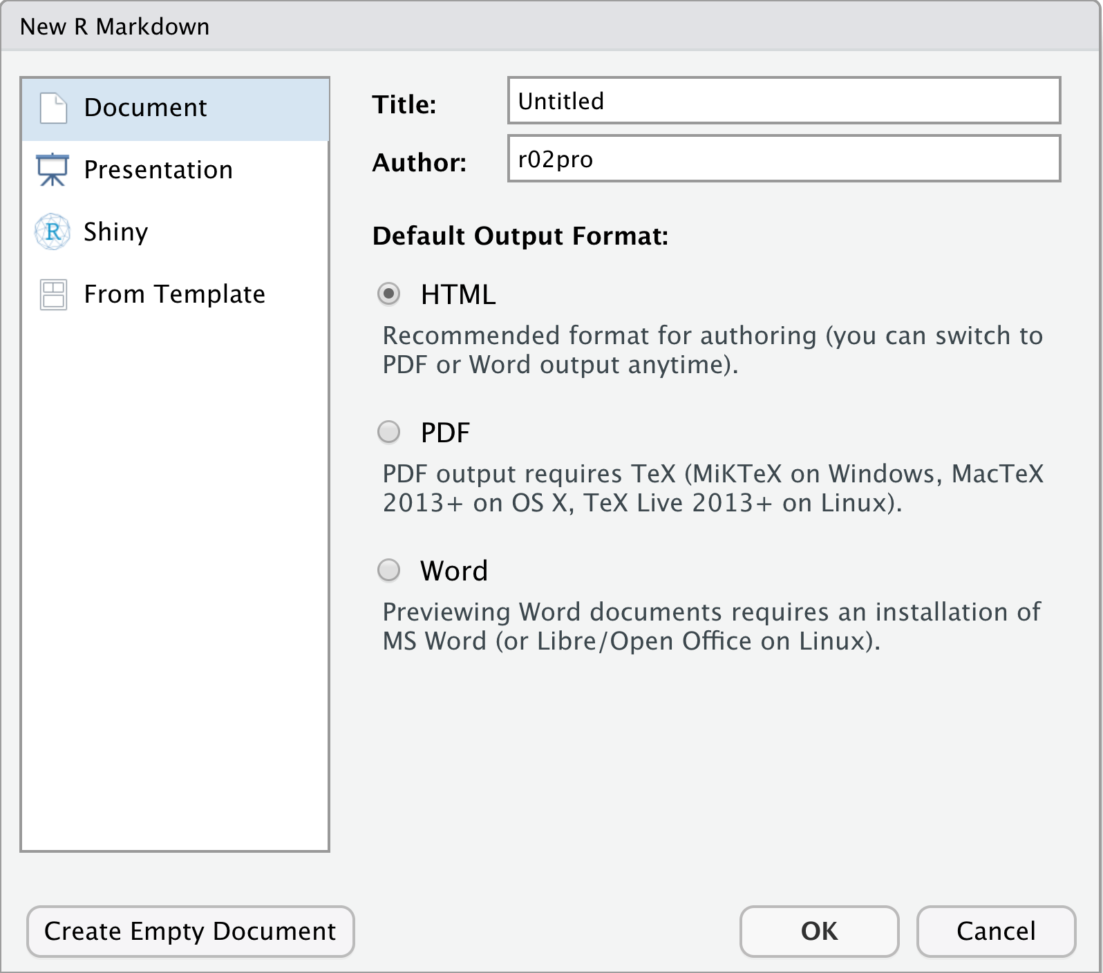
Figure 12.2: create a new R Markdown document (II)
Here, you can enter the Title and Author of the document, and select one of the output formats: HTML, PDF and Word. In our opinion, HTML is the recommended format for authoring. If you want to generate a PDF, you need to have a Tex installation, which would have already been installed if you write LaTex documents on the computer. If necessary, you can install TinyTeX with the R package tinytex.
install.packages("tinytex")
tinytex::install_tinytex()
A word of caution is needed here. We have seen a lot of people having issues with the installation of the Tex system. The exact cause is sometimes tricky to track. It could be the operating system, the physical location, existing software installed on the computer, or something else. If an error message shows up during the installation process, you are not alone. You could try to search the error message using a search engine. If generating PDF file is a must, as a last resort, you can first generate a word document and convert it into a pdf file afterward.
After clicking OK, you have created an R Markdown document with file extension .Rmd. You can save the file with a desired name on the disk by clicking the save button or using keyboard shortcut of saving files. Here, we use the name Lesson 10.1. It is clear to see the difference of file extension between R Markdown document and R script.
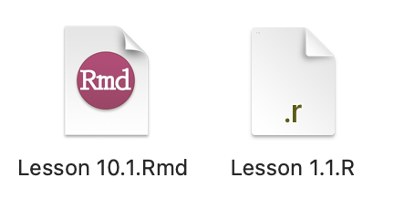
Figure 12.3: R Markdown vs. R Script
12.1.2 Knit the R Markdown document
To generate the final output document, you need to knit the .Rmd file. To do that, you can click the Knit button shown in the following figure.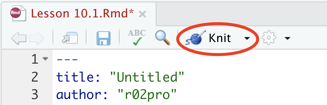
Figure 12.4: Knit button
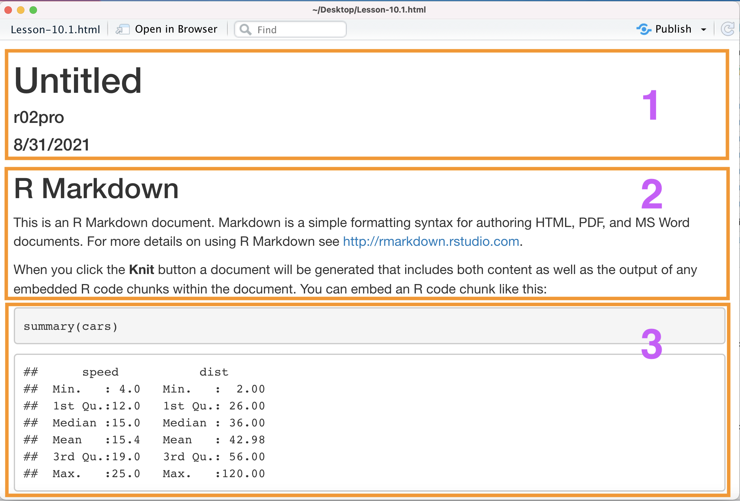
Figure 12.5: HTML document
A document consists of components three different types. The first type is the header of document, the second type is text, and the third type is related to codes and the results. Since the output document is rendered from the .Rmd file, the .Rmd file also has three type of components accordingly.
If you want to make any changes on the output document, you need to make the necessary changes on the .Rmd file and knit it again. Next, we introduce how to write an R Markdown document.
12.1.3 Write an R Markdown document
Unlike R script, you may notice that RStudio provides an example of the .Rmd file after creating an R Markdown document. It is then straightforward for you to get started by replacing the example with your own contents.
By now you know that there are three parts in the .Rmd file. Let’s go over them one by one.
a. YAML header
The first part is a YAML header (Yet Another Markup Language), which is a section of key: value pairs surrounded by --- marks, like below.
---
title: "Untitled"
author: "r02pro"
date: "8/31/2021"
output: html_document
---
It is used to specify the document information, including the title, author, date, and output format. The output: recognizes the following values:
- html_document, which will create HTML output (default)
- pdf_document, which will create PDF output
- word_document, which will create Word output
b. Text
After the YAML header, you can see some text. Unlike R script, you don’t need to use the pound sign # to write text in an R Markdown document. Indeed, you can write as if you are writing in a text editor, though R Markdown provides a rich collection of text formats, which will be discussed in Section 12.2.
c. Code Chunks
The last component type is related to R codes. Different from R script, the R code is usually contained in the code chunks in the .Rmd file. So what is a code chunk?
A code chunk is basically a collection of R codes surrounded by the chunk delimiters```{r} and ```. Let’s take a look at one code chunk as follows.

Figure 12.6: An R Code Chunk
In this code chunk, there is only one line of code summary(cars) which will output the summary statistics of the cars data set. If necessary, you can include any lines of codes inside each code chunk. Each chunk can be viewed as a unit that usually serves a particular purpose. Inside each code chunk, you can run the codes line by line by the keyboard shortcut Cmd + Enter / Ctrl + Enter. However, it is often more convenient to run the codes all at once using the keyboard shortcut Shift + Cmd + Enter / Shift + Ctrl + Enter, or press the Green arrow on the right of the code chunk.
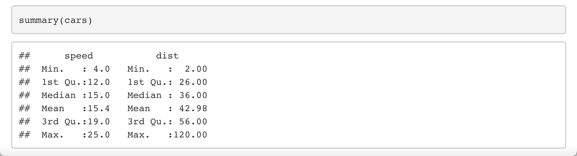
Figure 12.7: R code and the result
In addition to the R code, you may be wondering what do the arguments in the big parentheses { } work for. Here, we will introduce a few useful chunk options which control the behavior of each code chunk.
- “r cars” gives the code chunk the name “pressure,” which is useful to navigate between different chunks, and it is also necessary to give the code chunk a name if you want to cross reference the corresponding figure in the knitted document.
eval = FALSEprevents codes from being evaluated. This is useful when you want to show the code but don’t want to run it. Default value iseval = TRUE.include = FALSEprevents code and results from appearing in the knitted file. The code will still be evaluated. Default value isinclude = TRUE.echo = FALSEprevents code, but not the results from appearing in the knitted file. This is useful if you want to embed figures in the document without showing the code used to generate them. Default value isecho = TRUE.message = FALSEprevents messages that are generated by code from appearing in the knitted file. Default value ismessage = TRUE.warning = FALSEprevents warnings that are generated by code from appearing in the knitted file. Default value iswarning = TRUE.
There are many other available options in an R Markdown code chunk. You can refer to the webpage https://yihui.org/knitr/options/ for details.
Now let’s see some examples together. If you add the chunk optioneval = FALSE.

Figure 12.8: Add eval = FALSE
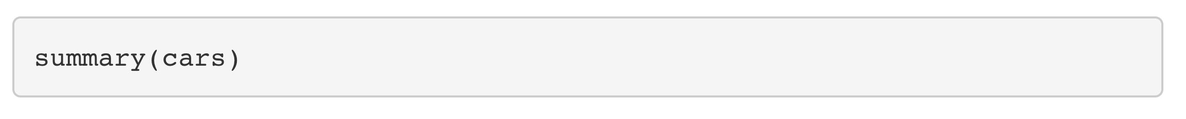
Figure 12.9: Only see the code
echo = FALSE,

Figure 12.10: Add echo = FALSE
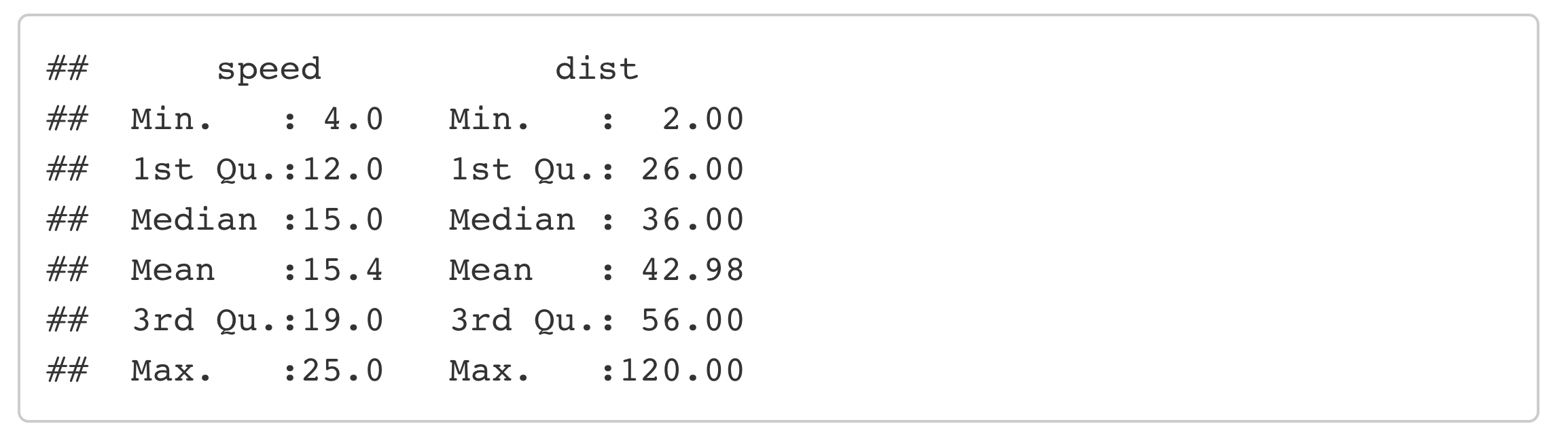
Figure 12.11: Only see the result
You can try to add other chunk options by yourself!
Lastly, if you have many code chunks that share some chunk options, it is very useful to set the global chunk options at the beginning of an R Markdown document. To do that, you can add the following chunk right after the YAML header.
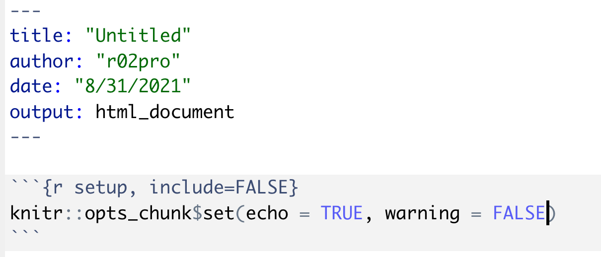
Figure 12.12: global chunk options
In this example, we set echo = TRUE and warning = FALSE. You can feel free to change their values and add other kinds of customization. In each subsequent chunk, this set of global chunk options will be inherited. Of course, you can add additional options in each chunk to add additional chunk options or overwrite the global chunk options. This may be reminiscent of the relationship between global and local aesthetic mappings introduced in Section 4.6.