4.19 Summary of Geoms & Grammatical Structure of ggplot()

In this section, we will have a concise review for using ggplot() to do data visualization.

4.19.1 Summarize all geoms

First, let’s summarize all the geoms we have covered.

Names	Funs	Section
One continuous variable (e.g. sale_price)
Histogram	geom_histogram(aes(x = sale_price))	4.12
Density	geom_density(aes(x = sale_price))	4.13
Boxplot	geom_boxplot(aes(x = "", y = sale_price))	4.14.2
Violin	geom_violin(aes(x = sale_price))	4.15
Errorbar	geom_errorbar(aes(x = "", y = sale_price), stat = "summary", fun.data = "mean_se")	4.16
One discrete variable (e.g. kit_qual)
Bar Chart	geom_bar(mapping = aes(x = kit_qual))	4.10
Pie Chart	geom_bar(aes(), stat = "identity") + coord_polar("y")	4.10.4
Two continuous variables (e.g. liv_area and sale_price)
Scatterplot	geom_point(mapping = aes(x = liv_area, y = sale_price))	4.2.2
Smoothline	geom_smooth(mapping = aes(x = liv_area, y = sale_price))	4.4
Line Plot	geom_line(mapping = aes(x = dt_sold, y = sale_price))	4.7
Two discrete variables (e.g. kit_qual and heat_qual):
Jiter Plot	geom_jitter(mapping = aes(x = kit_qual, y = heat_qual))	4.9.2
Count Plot	geom_count(mapping = aes(x = kit_qual, y = heat_qual))	4.9.3
One continuous variable and one discrete variable (e.g. kit_qual and sale_price):
Boxplot	geom_boxplot(aes(x = kit_qual, y = sale_price))	4.14.3

Note that in the summary, we are only using the basic geoms. Clearly, we can map variables to aesthetics or use facet_wrap() (in Section 4.17.1) or facet_grid() (in Section 4.17.2) to arrange the subplots into facets depending on the grouping variable(s).

There are more than 40 geoms in the ggplot2 package with many more geoms developed in other packages. So far, we’ve covered the most commonly used geoms. You can feel free to explore other geoms by doing an online search or looking at the documentation.

4.19.2 The grammatical structure of ggplot()

Next, we review the grammatical structure of ggplot().

Code	Info
ggplot(data = <DATA>) +	data to be used
<GEOM_FUNCTION>(	geom for generating the desirable plot
mapping = aes(<MAPPINGS>),	aesthetic mappings, this may include the x and y axes and other features like color, shape, fill, linetype, size, etc.
stat = <STAT>,	statistical transformation, for example, when we create the errorbar
position = <POSITION>) +	position, like stack, dodge, fill
<COORDINATE_FUNCTION> +	such as flipping the x and y axes
<FACET_FUNCTION> +	facet_wrap() and facet_grid(), create multiple plots for different subsets of the data
<SCALE_FUNCTION> +	customize the x and y breaks
<THEME_FUNCTION>	customize labels, title, and fonts

4.19.3 A complex ggplot() example

To conclude this chapter, let’s look at an example with all components.

library(r02pro)
library(tidyverse)
ggplot(data = na.omit(sahp)) +
  geom_bar(
    mapping = aes(x = kit_qual, fill = oa_qual > 5),
    stat = "count", #Default stat for geom_bar, can be removed
    position = "fill") +
  coord_flip() +
  facet_wrap(vars(house_style)) +
  scale_y_continuous(breaks = seq(from = 0, to = 1, by = 0.2)) +
  theme(plot.title = element_text(size = 24, color = "magenta")) +
  ylab("proportion") +
  ggtitle('A bar chart for the sahp dataset')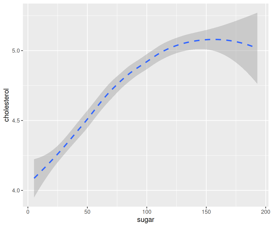

This plot shows a bar chart using the data sahp for the variable kit_qual, map the variable oa_qual > 5 to the fill aesthetic and with fill position, with the x and y coordinates flipped, faceted using the variable house_style, and with the breaks on the y axis, the title and its font, the label on the y axis being customized.