7.5 Create Grouped Summaries via group_by() and summarize()

7.5 Create Grouped Summaries via `group_by()` and `summarize()`

In Section 7.4, you learned how to create new variables as functions of the existing ones. For example, we created a variable representing the order of GDP per capita for each country in the year 2008. In this section, we will learn how to create summaries for each group of observations.

The dplyr package provides two useful functions to achieve this: namely group_by() which can group the observations according to the specified variables, and summarize() which create summaries for each group.

7.5.1 Create Summaries

To create summaries for a variable, you can use the summarize() function. Let’s compute the number of countries, the average population, and the median of the GDP per capita for all observations in the gm dataset for the year 2008.

library(r02pro)
library(tidyverse)
gm %>%
    filter(year == 2008) %>%
    summarize(n_countries = n(), ave_population = mean(population, na.rm = TRUE),
        q_GDP = median(GDP_per_capita, na.rm = TRUE))
#> # A tibble: 1 × 3
#>   n_countries ave_population q_GDP
#>         <int>          <dbl> <dbl>
#> 1         236         34848.  5.12

Note that here we use the n() function to count the number of countries. The mean() function computes the average of the population, and the median() function computes the median of the GDP per capita. The na.rm = TRUE argument is used to remove the missing values when computing the average and median.

7.5.2 Create Grouped Summaries

So far, we have learned to use summarize() to create summaries for all observations. In practical applications, it is often more useful to compute the summaries when the observations are grouped according to certain criteria. Let’s say we want to create the same summaries for each continent in the gm dataset.

gm %>%
    group_by(continent) %>%
    summarize(n_countries = n(), ave_population = mean(population, na.rm = TRUE),
        q_GDP = median(GDP_per_capita, na.rm = TRUE))
#> # A tibble: 6 × 4
#>   continent n_countries ave_population  q_GDP
#>   <chr>           <int>          <dbl>  <dbl>
#> 1 Africa          15051         19103.  0.984
#> 2 Americas        10578         16009.  5.26 
#> 3 Asia            13764         53912.  3.41 
#> 4 Europe          11439         13590. 19.1  
#> 5 Oceania          3446          2419.  2.87 
#> 6 <NA>            11253          5008. 11.8

From the output, you can see that the summaries are created for each continent. The group_by() function is used to group the observations according to the continent variable. Then, the summarize() function is used to create the summaries for each group.

Let’s now do another example. We want to find the top 5 countries with the highest life expectancy in the year 2006 for each continent.

gm %>%
    filter(year == 2006, !is.na(continent)) %>%
    group_by(continent) %>%
    top_n(5, life_expectancy) %>%
    select(country, life_expectancy) %>%
    arrange(continent, desc(life_expectancy))
#> Adding missing grouping variables:
#> `continent`
#> # A tibble: 25 × 3
#> # Groups:   continent [5]
#>    continent country    life_expectancy
#>    <chr>     <chr>                <dbl>
#>  1 Africa    Libya                 76  
#>  2 Africa    Tunisia               75.7
#>  3 Africa    Mauritius             73.8
#>  4 Africa    Algeria               73.6
#>  5 Africa    Cape Verde            73.2
#>  6 Americas  Canada                80.9
#>  7 Americas  Costa Rica            80.3
#>  8 Americas  Cuba                  78.5
#>  9 Americas  Panama                78.5
#> 10 Americas  Chile                 78.4
#> # … with 15 more rows

In this example, we first filter the observations for the year 2006 and remove the missing values in the continent variable. Then, we group the observations according to the continent variable. The top_n() function is used to select the top 5 countries with the highest life expectancy for each continent. Finally, we select the country and life_expectancy variables and arrange the observations according to the continent and the life expectancy in descending order.

Finally, let’s say we want to visualize the trend of the average GDP per capita for each continent from 1998 to 2018.

gm %>%
    filter(year >= 1998 & year <= 2018 & !is.na(continent)) %>%
    group_by(continent, year) %>%
    summarize(ave_GDP = median(GDP_per_capita, na.rm = TRUE)) %>%
    ggplot(aes(x = year, y = ave_GDP, color = continent)) + geom_smooth(se = FALSE) +
    labs(title = "Trend of Average GDP per Capita by Continent", x = "Year", y = "Average GDP per Capita")
#> `summarise()` has grouped output by
#> 'continent'. You can override using the
#> `.groups` argument.
#> `geom_smooth()` using method = 'loess'
#> and formula = 'y ~ x'

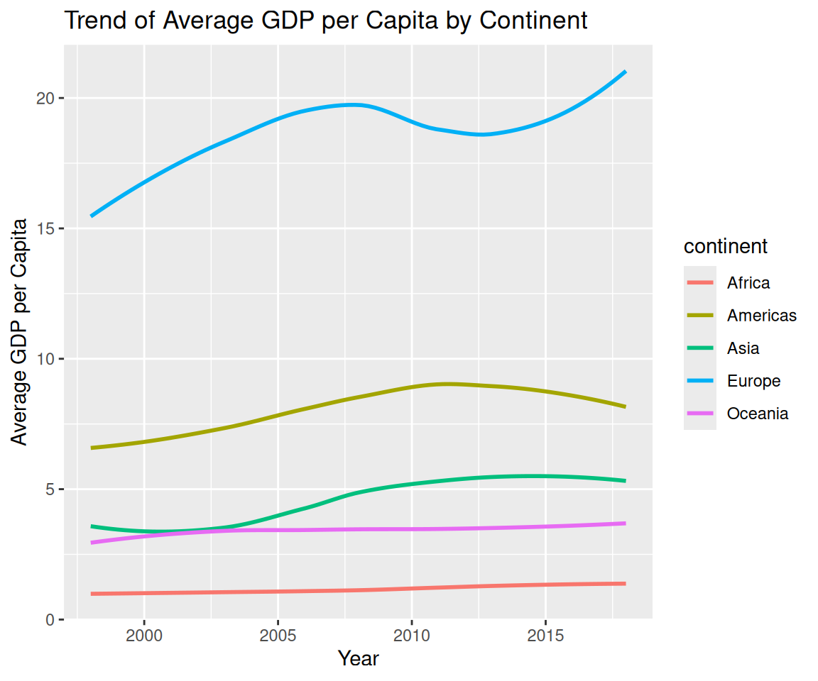
Here, we first filter the observations for the years from 1998 to 2018 and remove the missing values in the continent variable. Then, we group the observations according to the continent and year variables. The summarize() function is used to compute the median of the GDP per capita for each group. Finally, we create a smoothline fit to visualize the trend of the average GDP per capita for each continent from 1998 to 2018.

7.5.3 Exercises

Using the ahp dataset and the pipe operator for the following exercises.

For each month when the house was sold, summarize the 1st and 3rd quartile of the sale price. Then, create a scatterplot between the month (x-axis) and the quartile of the sale price with different colors for 1st and 3rd quantile. Explain the findings from the figure.
Someone has a conjecture that when sold, the houses that are less than or equal to 30 years old have a higher sale price than the houses that are more than 30 years old. Show whether this is true in terms of maximum price, median price, and the minimum price for the houses in each group.