5.2 Importing Data from Delimited Files

Knowing how to export data into delimited files, let’s see how to import data from the delimited files.

5.2.1 Import .csv Files using `read_csv()`

To import .csv files, we can use the function read_csv() in the readr package, which is a sub-package of tidyverse. If you have already installed tidyverse, you can directly load the readr package.

After loading the readr package, you can try to import the data from “my_animals.csv,” which we created in Section 5.1.3. Please make sure the .csv file is located in the current working directory. Otherwise, you need to change the working directory to where the file is located by the methods introduced in Section 5.1.1.

library(readr)
my_animals <- read_csv("my_animals.csv")
#> Rows: 7 Columns: 3
#> ── Column specification ────────────────────────────────────────────────────────
#> Delimiter: ","
#> chr (2): ani_char, conditions
#> dbl (1): dig_num
#> 
#> ℹ Use `spec()` to retrieve the full column specification for this data.
#> ℹ Specify the column types or set `show_col_types = FALSE` to quiet this message.

We can see that there is a message showing the Column specification during the import process. In particular, we see dig_num is of type double, and both ani_char and cond_fac are both of type character. We can also check the value of my_animals and its structure.

my_animals
#> # A tibble: 7 × 3
#>   dig_num ani_char conditions
#>     <dbl> <chr>    <chr>     
#> 1       7 sheep    Excellent 
#> 2       6 pig      Good      
#> 3       5 monkey   N         
#> 4       4 pig      Fair      
#> 5       3 monkey   Good      
#> 6       2 <NA>     Good      
#> 7       1 pig      Excellent
str(my_animals)
#> spec_tbl_df [7 × 3] (S3: spec_tbl_df/tbl_df/tbl/data.frame)
#>  $ dig_num   : num [1:7] 7 6 5 4 3 2 1
#>  $ ani_char  : chr [1:7] "sheep" "pig" "monkey" "pig" ...
#>  $ conditions: chr [1:7] "Excellent" "Good" "N" "Fair" ...
#>  - attr(*, "spec")=
#>   .. cols(
#>   ..   dig_num = col_double(),
#>   ..   ani_char = col_character(),
#>   ..   conditions = col_character()
#>   .. )
#>  - attr(*, "problems")=<externalptr>

We can see that the tibble my_animals is generated along with the correct column types. In order to introduce the various options associated with read_csv() function, let’s move on to the topic of inline .csv files next.

5.2.2 Read Inline .csv Files

The read_csv() function not only can read files into R, it also accept inline input as its argument. While the inline input may not be commonly used in practice, it is particularly useful for learning how to use the function. Let’s see an example.

read_csv("x,y,z
          1,3,5
          2,4,6")
#> Rows: 2 Columns: 3
#> ── Column specification ────────────────────────────────────────────────────────
#> Delimiter: ","
#> dbl (3): x, y, z
#> 
#> ℹ Use `spec()` to retrieve the full column specification for this data.
#> ℹ Specify the column types or set `show_col_types = FALSE` to quiet this message.

You can see that a tibble is generated with 2 rows and 3 columns with the column names being x, y and z. From the argument, we can see that by default, the first row of the input data will be interpreted as the column names.

a. No column names

If the first row of the input data doesn’t correspond to the variable names, you need to set col_names = FALSE as an additional argument in read_csv().

read_csv("x,y,z
          1,3,5
          2,4,6", col_names = FALSE)
#> Rows: 3 Columns: 3
#> ── Column specification ────────────────────────────────────────────────────────
#> Delimiter: ","
#> chr (3): X1, X2, X3
#> 
#> ℹ Use `spec()` to retrieve the full column specification for this data.
#> ℹ Specify the column types or set `show_col_types = FALSE` to quiet this message.

Now, a tibble of 3 rows and 3 columns was generated, with the column names being X1, X2, and X3. Note that these are the naming convention in the function when you don’t supply the column names in the file. Another thing worth mentioning is that all three variables are of character types, due to the fact that there are character values for all variables (x, y, and z).

b. Skip the first few lines

Sometimes, the first few lines of your data file may be descriptions of the data, which you want to skip when importing into R. We can set the skip argument in the read_csv() function to skip a certain number of lines.

read_csv("The first line 
          The second line
          The third line
          x,y,z
          1,3,5", skip = 3)
#> Rows: 1 Columns: 3
#> ── Column specification ────────────────────────────────────────────────────────
#> Delimiter: ","
#> dbl (3): x, y, z
#> 
#> ℹ Use `spec()` to retrieve the full column specification for this data.
#> ℹ Specify the column types or set `show_col_types = FALSE` to quiet this message.

It is clear from the result that the first 3 lines of the input data is skipped.

5.2.3 Handling Missing Values

In many real data sets, we may have missing values. You may recall that R uses NA to represent the missing values. If the data set was prepared by an R user, it probably already uses NA to represent all missing values. In this case, life is easy since read_csv() will automatically interpret all NAs as missing values.

read_csv("x,y,z
          999,3,5
         NA,-999,6")
#> Rows: 2 Columns: 3
#> ── Column specification ────────────────────────────────────────────────────────
#> Delimiter: ","
#> dbl (3): x, y, z
#> 
#> ℹ Use `spec()` to retrieve the full column specification for this data.
#> ℹ Specify the column types or set `show_col_types = FALSE` to quiet this message.

In a typical application, however, the person who prepared the data may use other strings to represent missing values. For example, if 999 and -999 are used as the indicators for missing values, you can set the argument na to be the vector containing those values, along with the default NA.

read_csv("x,y,z
          999,3,5
         999,-999,6", na = c("999","-999", NA))
#> Rows: 2 Columns: 3
#> ── Column specification ────────────────────────────────────────────────────────
#> Delimiter: ","
#> dbl (2): y, z
#> lgl (1): x
#> 
#> ℹ Use `spec()` to retrieve the full column specification for this data.
#> ℹ Specify the column types or set `show_col_types = FALSE` to quiet this message.
#> # A tibble: 2 × 3
#>   x         y     z
#>   <lgl> <dbl> <dbl>
#> 1 NA        3     5
#> 2 NA       NA     6

You can see from the output tibble that all the missing values are now denoted as NA.

Note that the quotation marks around 999 and -999 are necessary since the na argument is expecting a character vector.

read_csv("x,y,z
          999,3,5
         999,-999,6", na = c(999,-999, NA))
#> Error in enc2utf8(na): argument is not a character vector

You can see an error message, stating that it is expecting character values, but got double values.

5.2.4 Importing Data From a Delimited File

You now know how to import data from a .csv file using the read_csv() function. More generally, read_delim() allows us to import data from a delimited file with any chosen delimiter. The usage of read_delim() is almost identical to read_csv(), except that it has an additional argument delim, which specifies the delimiter to be used. Let’s see the following example with * as the delimiter. Note that we are using the “my_animals_star.csv” file generated in Section 5.1.4.

my_animals <- read_delim("my_animals_star.csv", delim = "*")

5.2.5 Import Data Using the Menu

Besides writing codes involving read_csv() or read_delim() to import data, you can also take advantage of the interactive menu RStudio provides.

To do this, you can click on the Import Dataset button in the Environment panel on the top right of RStudio shown in the following figure.

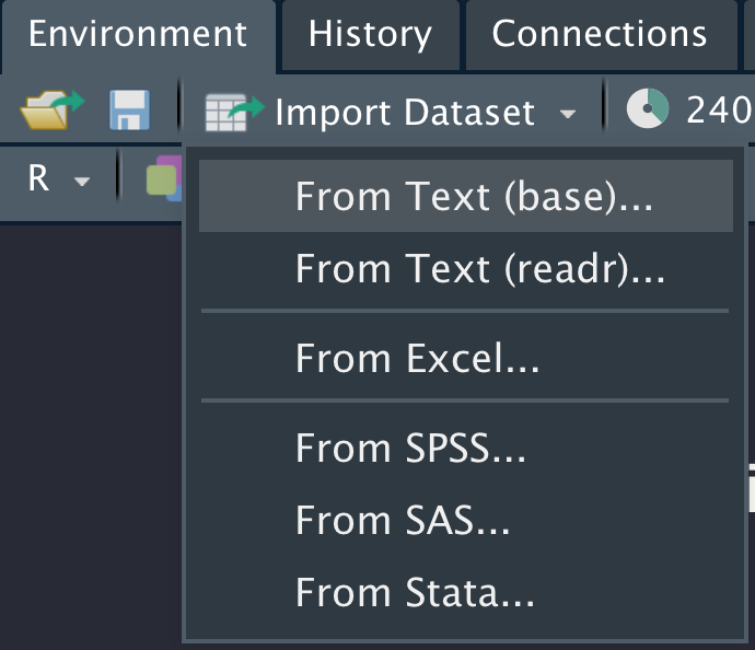
Figure 5.4: Import Dataset Menu

Here, you can see quite a few options which are summarized in the following table.

Table 5.1: Import Data from Menu
Choice	Name
From Text (readr)	Delimited Files (.csv, .txt, and others)
From Excel	Excel Files (.xls and .xlsx)
From SPSS	SPSS Files (.sav)
From SAS	SAS Files (.sas7bdat and.sas7bcat)
From Stata	Stata Files (.dta)

We will focus on importing delimited files in this section. We will cover importing Excel files in Section 5.3. Working with SPSS, SAS, and Stata files will be covered in Section 5.4.

For importing a .csv file, .txt file, or any other file with a delimiter, you can choose the From Text (readr) option. Then, you can click Browse… and select the data file. We will select the “my_animals_star.csv” file.

After a file is selected, you can see the Data Preview which showing the first several rows of the data. Note that the first row shows the column names and their associate types in parentheses. For each column, you can click the drop-down menu after the type to change its type.

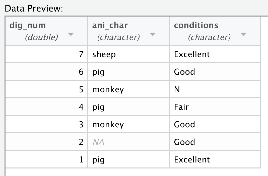
Figure 5.5: Import Data Preview

From this figure, you can see that the preview only shows one column named “dig_num*ani_char*conditions.” Apparently, the separator “*” is not properly interpreted during the process.

Besides the data preview, there is also the Code Preview window on the bottom right. The Code Preview shows the R Codes which were run to read the data into R and display it in the Data Preview.

Figure 5.6: Code Preview

Clearly, the default function is the read_csv() function, which is not appropriate here.

To fix this problem, we can look at the Import Options in the bottom left area.

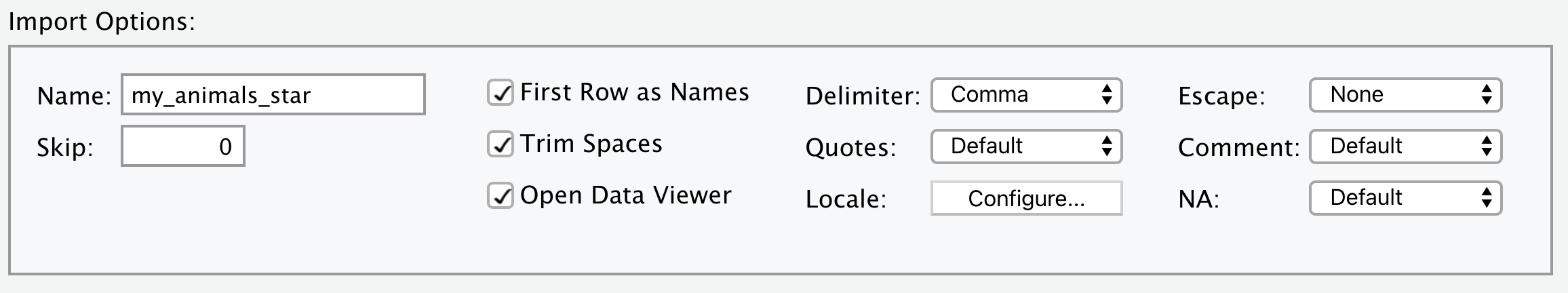
Figure 5.7: Import Options

Let’s summarize a few commonly used options, their corresponding arguments in the read_csv() or read_delim() function, and meanings.

Table 5.2: Menu Options and its Corresponding Arguments in `read_delim()` and Meanings
Option	Argument	Meaning
Name		The object name you would like to assign to.
Skip	`skip`	The number of rows to skip at the beginning of the file.
First Row as Names	`col_names`	Whether you want to use the first row as column names. `TRUE` or `FALSE`.
Delimiter	`delim`	The delimiter of the data file.
Comment	`comment`	The character indicating the starting of comment. The contents after the comment character will be ignore in each line.
NA	`na`	The way NA is represented in the data file.
Code Preview		The R code to be executed for importing the data

In our case, we will change the value of “Delimiter” to “*” (Note that you need to select “Other..” and enter “*” manually.)

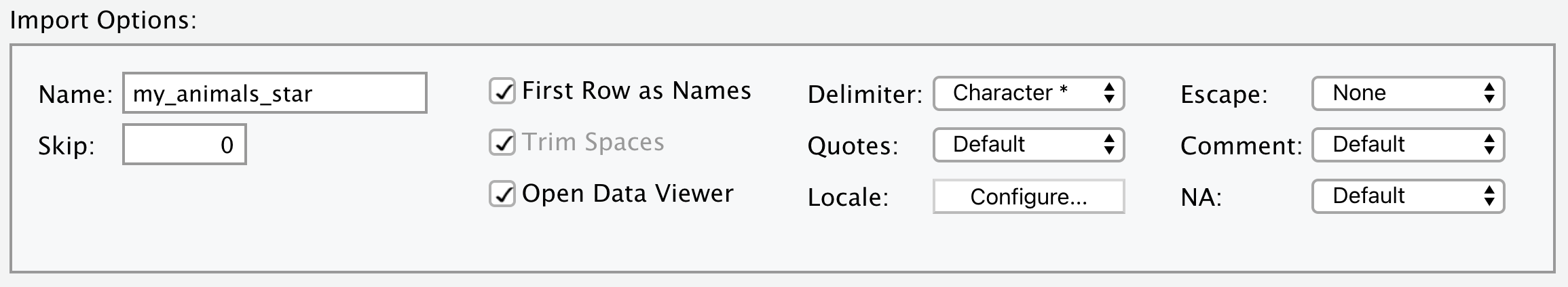
Figure 5.8: Import Options (Star)

Note that when you change the delimiter, the Data Preview window also change correspondingly.

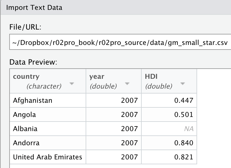
Figure 5.9: Data Preview (Star)

After changing the delimiter to \*, we are seeing the expected data with three columns: dig_num, ani_char, and conditions.

The code in the Code Preview window will change accordingly, which is a great way to learn on how they work. The new codes in the Code Preview window is as below.

library(readr)
my_animals_star <- read_delim("~/Dropbox/R/my_animals_star.csv", 
    "*", escape_double = FALSE, trim_ws = TRUE)
View(my_animals_star)

5.2.6 Exercises

For the “my_data_na.csv” file you created in Exercise 2 in Section 5.1, write R code to read the file into an object with name my_data.
First, look at the code below.

d1 <- read_csv("x,y,z
          1,3,5
          2,4,6", col_names = FALSE)

Which of the following are the column names of the d1?

X1, X2, and X3
x, y, and z

First, look at the code below.

d1 <- read_csv("The first line 
          The second line
          The third line
          x,y,z
          1,3,5")

What will be the column name(s) of the d1?