5.6 Smoothline Fits

Now, you know how to create scatterplots and line plots with many possible customizations via specifying different aesthetics. In addition to scatterplots, a very useful type of plots that can capture the trend of pairwise relationship is the smoothline fits.

5.6.1 Creating Smoothline Fits using `geom_smooth()`

To create a smoothline fit, you can use the geom_smooth() function in the ggplot2 package. Let’s say you want to find the trend between cholesterol and sugar in the gm2004 dataset.

library(ggplot2)
library(r02pro)
ggplot(data = gm2004) + geom_smooth(mapping = aes(x = sugar, y = cholesterol))
#> `geom_smooth()` using method = 'loess'
#> and formula = 'y ~ x'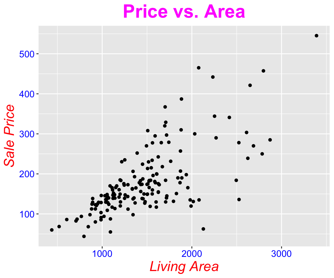

Perhaps it is helpful to review the code for generating a scatterplot between cholesterol and sugar.

ggplot(data = gm2004) + geom_point(mapping = aes(x = sugar, y = cholesterol))

We can see that the only difference between these two codes is the use of different geoms. In fact, the mechanism of geom_smooth() is that it fits a smooth line according to the points of the given variable pair. By default, it uses the loess method (locally estimated scatterplot smoothing), which is a popular nonparametric regression technique. In addition to the smoothline, it also generates a shaded area, representing the confidence interval around the fitted smoothline.

5.6.2 Constant-Valued Aesthetics in Smoothline Fits

Just like in scatterplots (Section 5.2), you can also set Constant-Valued Aesthetics for smoothline fits.

a. Confidence Interval (Hide or Display)

As mentioned before, the default smoothline fit display a confidence interval around the smooth curve. To hide this shaded area, you can add the argument se = FALSE as a Constant-Valued aesthetic.

ggplot(data = gm2004) + geom_smooth(mapping = aes(x = sugar, y = cholesterol), se = FALSE)
#> `geom_smooth()` using method = 'loess'
#> and formula = 'y ~ x'

b. Confidence Interval Level

The default confidence interval is at 95% level. To control the level, you can set the aesthetic level to a desired value.

ggplot(data = gm2004) + geom_smooth(mapping = aes(x = sugar, y = cholesterol), level = 0.9)
#> `geom_smooth()` using method = 'loess'
#> and formula = 'y ~ x'

c. Smoothing Method

In addition to the default loess method for smoothline fit, geom_smooth() also provides other smoothing methods. We can set the method aesthetic to change the smoothing method. For example, method = "lm" represents a linear line fit.

ggplot(data = gm2004) + geom_smooth(mapping = aes(x = sugar, y = cholesterol), method = "lm")
#> `geom_smooth()` using formula = 'y ~ x'

d. Color

Similar to Scatterplot, you can also set color to change the color of the line. Note that the color aesthetic is available for almost all geoms.

ggplot(data = gm2004) + geom_smooth(mapping = aes(x = sugar, y = cholesterol), color = "violet")
#> `geom_smooth()` using method = 'loess'
#> and formula = 'y ~ x'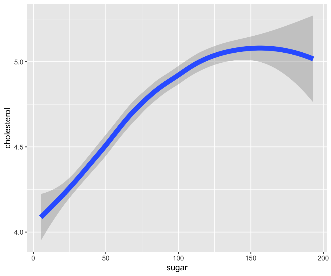

e. Size

Similar to Scatterplot, you can also set the size aesthetic. While the size controls the size of the points in a scatterplot, the size aesthetic controls the width of the smoothline.

ggplot(data = gm2004) + geom_smooth(mapping = aes(x = sugar, y = cholesterol), size = 3)
#> `geom_smooth()` using method = 'loess'
#> and formula = 'y ~ x'

f. Line Type

Another useful aesthetic that was not applicable in geom_point() is linetype, which controls the linetypes for each smoothline. The collection of different linetypes is available in Figure 5.3.

ggplot(data = gm2004) + geom_smooth(mapping = aes(x = sugar, y = cholesterol), linetype = 2)
#> `geom_smooth()` using method = 'loess'
#> and formula = 'y ~ x'

Note that it is common to use multiple constant-valued aesthetics.

ggplot(data = gm2004) + geom_smooth(mapping = aes(x = sugar, y = cholesterol), color = "purple",
    size = 2, method = "lm", level = 0.99, linetype = 2)
#> `geom_smooth()` using formula = 'y ~ x'

This generates a smoothline fit with purple color, line width 2, linear smoothing, 0.99 confidence level, and dashed line.

5.6.3 Local Aesthetics Mapping in Smoothline Fits

As in scatterplots (Section 5.3), you can also map variables to aesthetics in smoothline fits.

a. Group

When we map a variable to the group aesthetic, geom_smooth will first divide all the data points into different groups according to the variable value, and then fit a separate smoothline for each group.

ggplot(data = gm2004) + geom_smooth(mapping = aes(x = sugar, y = cholesterol, group = gender))
#> `geom_smooth()` using method = 'loess'
#> and formula = 'y ~ x'

You can see that two smoothlines are generated. However, it is not clear from the plot which group each smoothline corresponds to. To better differentiate the two groups, you can map the variable to other aesthetics like color.

b. Color

As in geom_point(), we can map the variable to the color aesthetic.

ggplot(data = gm2004) + geom_smooth(mapping = aes(x = sugar, y = cholesterol, color = gender))
#> `geom_smooth()` using method = 'loess'
#> and formula = 'y ~ x'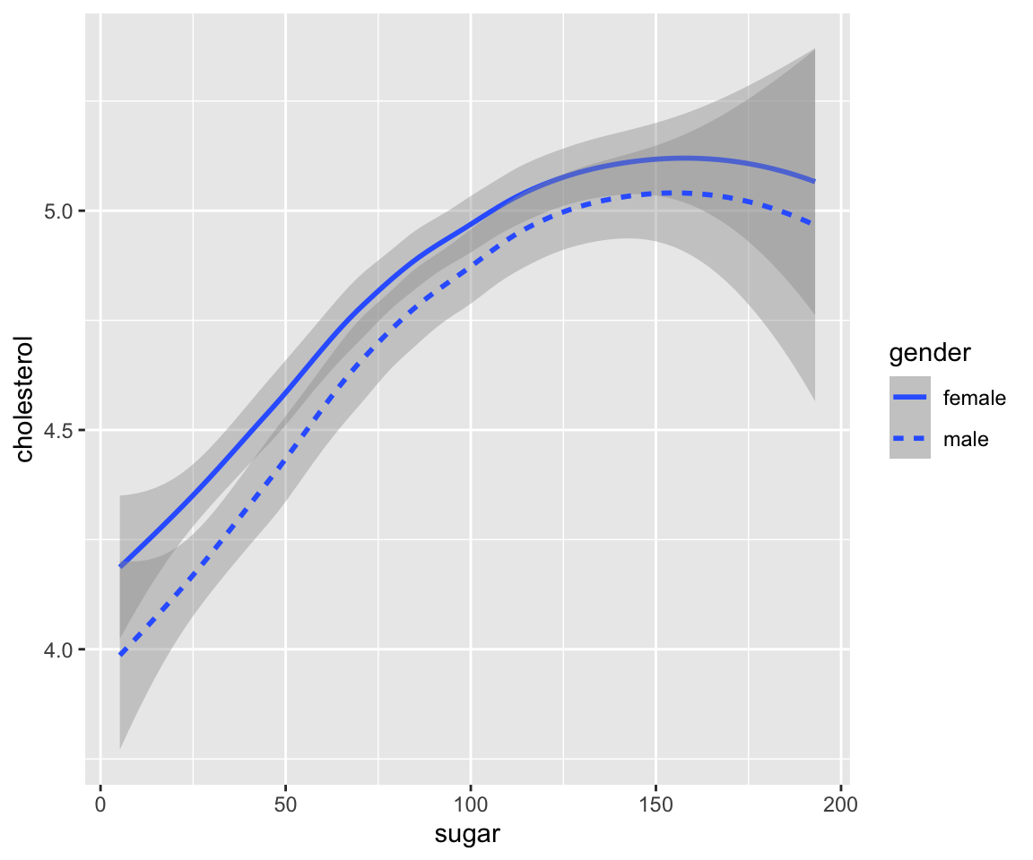

This is a more informative plot than the one using group aesthetic as you can see the two smoothlines have different colors according to the value of gender. We can observe that when the value of sugar is low, it appears that female has a larger cholesterol value than male and the difference becomes smaller as the sugar value increases.

c. Line Type

We can also use different line types to differentiate a variable by the linetype aesthetic.

ggplot(data = gm2004) + geom_smooth(mapping = aes(x = sugar, y = cholesterol, linetype = gender))
#> `geom_smooth()` using method = 'loess'
#> and formula = 'y ~ x'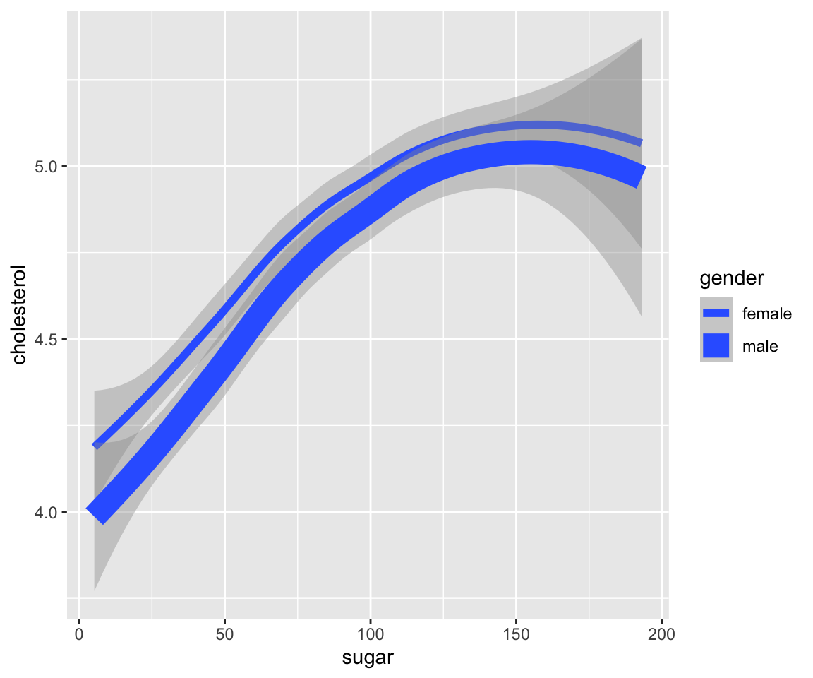

The plot shows a dashed line for the smoothline corresponding to gender = "male", and a solid line for the smoothline corresponding to gender == "female".

d. Size

You can also map gender to the size aesthetic, which controls the width of each smoothline fit.

ggplot(data = gm2004) + geom_smooth(mapping = aes(x = sugar, y = cholesterol, size = gender))
#> `geom_smooth()` using method = 'loess'
#> and formula = 'y ~ x'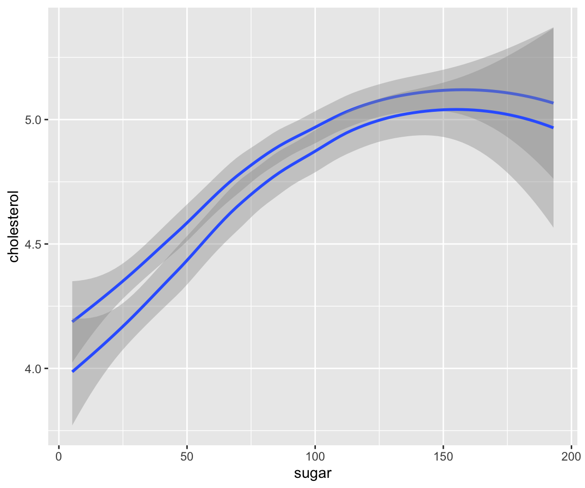

Note that similar to geom_point(), you can see a warning message: “Using size for a discrete variable is not advised.”

It is worth to mention that shape is not a valid aesthetic for geom_smooth as it doesn’t make sense to talk about the shape of a line.

ggplot(data = gm2004) + geom_smooth(mapping = aes(x = sugar, y = cholesterol, shape = gender))
#> `geom_smooth()` using method = 'loess'
#> and formula = 'y ~ x'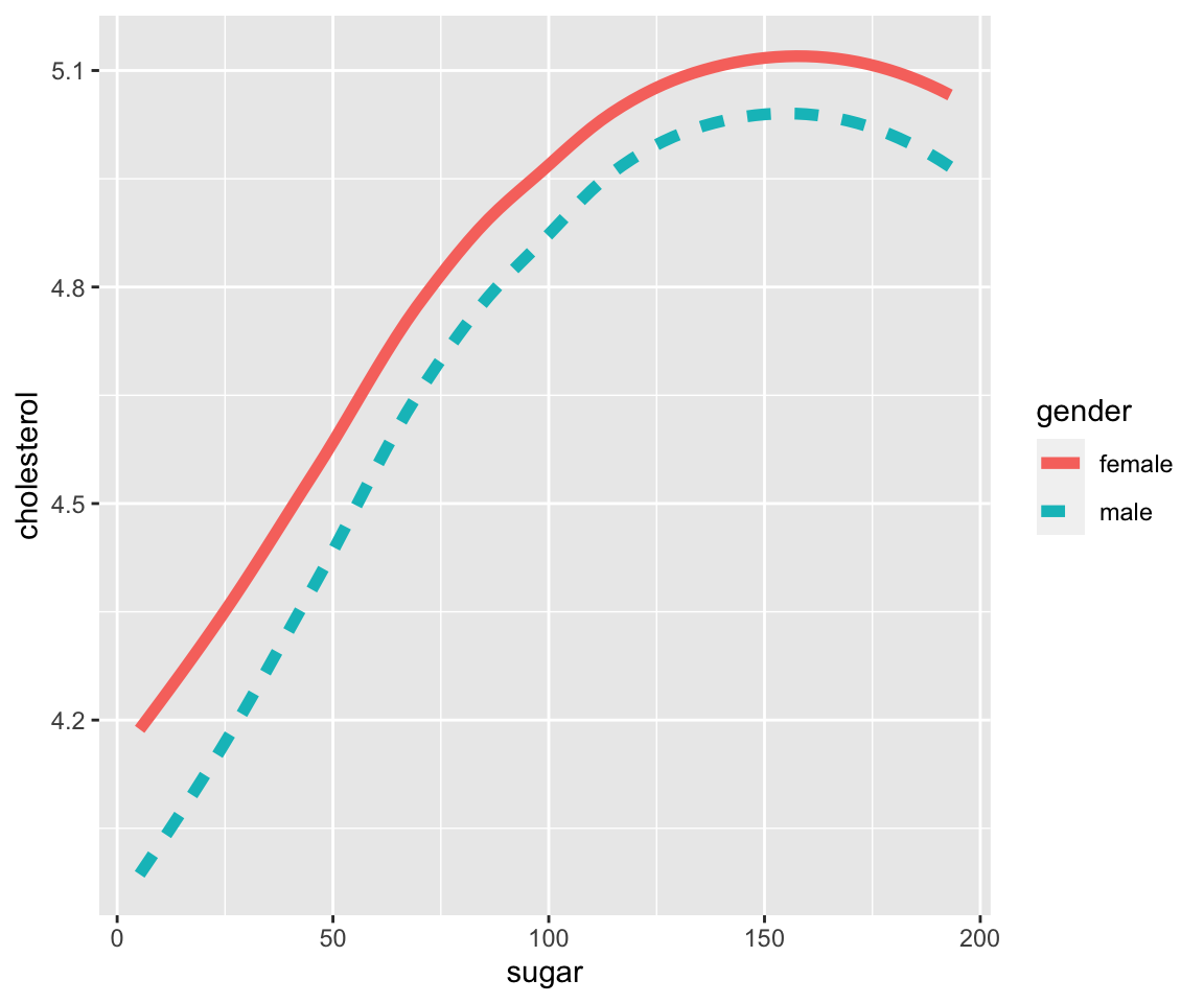

When you try to map a variable to the shape aesthetic, geom_smooth() will show a warning message “Warning: Ignoring unknown aesthetics: shape”, and use the group aesthetic instead.

Naturally, you can mix different local aesthetic mappings as well as different constant-valued aesthetics on the same plot.

ggplot(data = gm2004) + geom_smooth(mapping = aes(x = sugar, y = cholesterol, color = gender,
    linetype = gender), size = 2, se = FALSE)
#> `geom_smooth()` using method = 'loess'
#> and formula = 'y ~ x'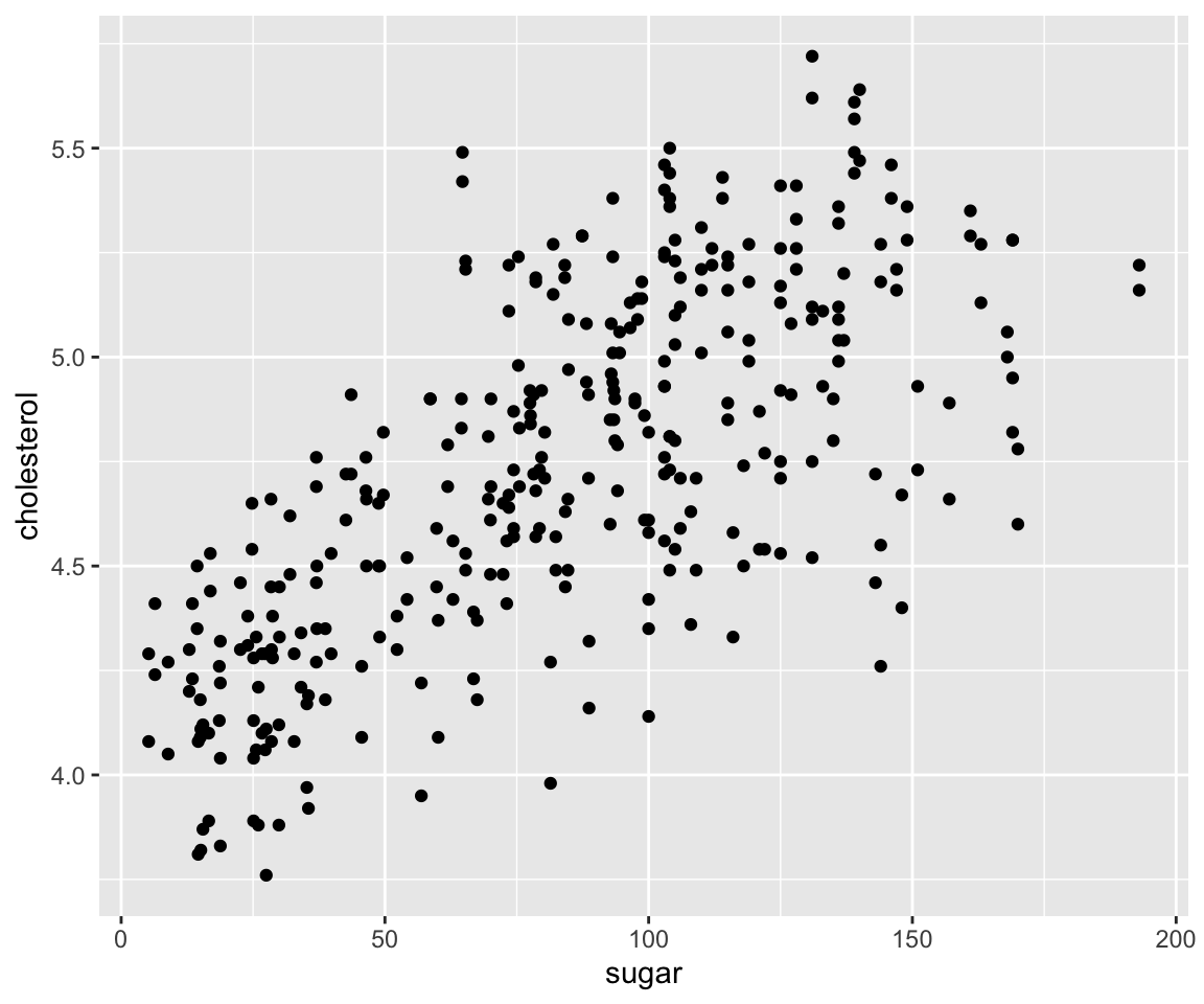

5.6.4 Exercises

Using the sahp dataset with the ggplot2 package, answer the following questions.

Create a smoothline fit to visualize the relationship between lot_area (on the x-axis) and sale_price (on the y-axis).
Create several smoothlines with different colors corresponding to the value of kit_qual to visualize the relationship between lot_area (on the x-axis) and sale_price (on the y-axis).
Create smoothlines without confidence interval around and with different linetypes to distinguish whether the house has more than 2 bedrooms to visualize the relationship between lot_area (on the x-axis) and sale_price (on the y-axis) .