1.2 Use R as a Fancy Calculator

After learning how to run codes in R, we will introduce how to use R as a fancy calculator.

1.2.1 Add comments using “#”

Before we get started, the first item we will cover is adding comments for codes. In R, you can use the hash character # at any position of a given line to initiate a comment, and anything after # will be ignored by R. Let’s see an example,

6 - 1/2  # first calculate 1/2=0.5, then 6-0.5=5.5
#> [1] 5.5

By running this line of code (either in the console or in the editor!), you will get a value of 5.5, which is the answer of 6 - 1 / 2. As demonstrated, R will not run syntax after the hash character #. Commands and strings after the # are notations or explanations that can make codes easier to understand. Here, the comment informs you the operation order of previous code: the division is calculated before the subtraction.

In general, adding comments to codes is a very good practice, as it greatly increases readability and make collaboration easier. We will also add necessary comments in our codes to help you learn R.

1.2.2 Basic calculation

Now let’s start to use R as a calculator! In the previous section we introduced operations such as addition, subtraction, multiplication, division, as well as the combination of multiple basic operations. Additionally, you can also calculate the square root, absolute value and the sign of a number.

Operation	Explanation
1 + 2	addition
1 - 2	subtraction
2 * 4	multiplication
2 / 4	division
6 - 1 / 2	multiple operations
sqrt(100)	square root
abs(-3)	absolute value
sign(-3)	sign

1.2.3 Get help in R

While the first seven operations in the above table look intuitive, you may be wondering, what does the sign() function mean there? Is that a stop sign?

Sometimes, you may have no idea how a particular function works. Fortunately, R provides a detailed documentation for each function.

a. Ask for help

First, we will introduce how to ask for help in R, and below are three common ways to seek for more information.

Use a question mark followed by the function name, e.g. ?sign
Use help function, e.g. help(sign)
Use the help window in RStudio, as shown in Figure 1.16. The help window is the panel 4 of Figure 1.4 in Section 1.1. Then type in the function name in the box to the right of the magnifying glass and press return.

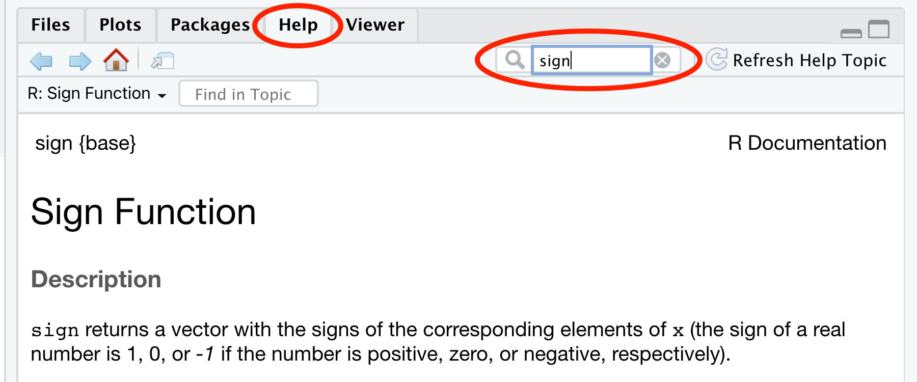
Figure 1.16: Ask for help

b. Documentation for functions

After using the above operations to ask for help in R, you can get the documentation of the function in the help window. The documentation consists of different parts, let’s take the sign() function as an example (Figure 1.17),

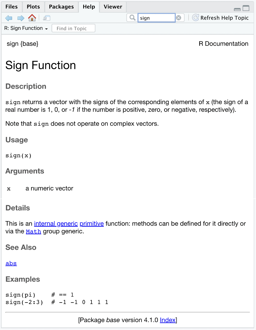
Figure 1.17: Documentation for function

This documentation contains the following parts:

Description: A text-format introduction of the function of interest. The introduction describes the function’s mechanism, the acceptable input and output types, and some notes of the function.
Usage: The way the function looks like.
Arguments: A detailed description of the input.
Details: A detailed description of the function, including the background, some complicated usage, and special cases of the function.
See Also: Some functions related or similar to this function.
Examples: Sample codes and their corresponding answers. You can simply copy codes in the Examples part and run them in the editor or in the console. Note that all words after # are comments and will be ignored by R.

Here, from the documentation of the sign() function, you will know that the sign() function can return the signs of numbers, which means it will return 0 for zero, return 1 for positive numbers, and return -1 for negative numbers.

The documentation of different functions can contain different parts, we will give you the introduction of other functions in the following sections.

1.2.4 Approximation

Next, let’s move on to the approximation in R. When computing 7 / 3, the answer is not a whole number as 7 is not divisible by 3. Approximation will come in handy under such circumstances. Let’s take 7 / 3 as the example.

a. Get the integer part and the remainder

Code	Name
7%/%3	integer division
7%%3	modulus

We all know that 7 = 3 * 2 + 1. So the integer division will pick up the integer part, which is 2 here; and the modulus will get the remainder, which is 1.

b. Get the nearby integer

floor(7/3)
#> [1] 2
ceiling(7/3)
#> [1] 3

Since 2 <= 7/3 <= 3, you can use the floor function to find the largest integer <= 7/3, which is 2; and the ceiling function gives the smallest integer >= 7/3, which is 3.

c. Round to the nearest number

round(7/3)
#> [1] 2
round(7/3, digits = 3)
#> [1] 2.333

The round() function follows the rounding principle. By default, you will get the nearest integer to 7 / 3, which is 2. If you want to control the approximation accuracy, you can add a digits argument to specify how many digits you want after the decimal point. Here you will get 2.333 after adding digits = 3.

1.2.5 Power & logarithm

You can also use R to do power and logarithmic operations.

Generally, you can use ^ to do power operations. For example, 10^5 will give us 10 to the power of 5. Here, 10 is the base value, and 5 is the exponent. The result is 100000, but it is shown as 1e+05 in R. That’s because R uses the so-called scientific notation.

scientific notation: a common way to express numbers which are too large or too small to be conveniently written in decimal form. Generally, it expresses numbers in forms of $m \times 10^n$ and R uses the e notation. Note that the e notation has nothing to do with the natural number $e$ . Let’s see some examples, $\begin{align} 1 \times 10^5 &= \mbox{1e+05}\\ 2 \times 10^4 &= \mbox{2e+04}\\ 1.2 \times 10^{-3} &= \mbox{1.2e-03} \end{align}$

Another thing to note is that we don’t use commas when writing a big number in R as we do in reports and essays. For example, we need to write 1000000 for a million instead of 1,000,000.

In mathematics, the logarithmic operations are inverse to the power operations. If $b^y = x$ and you only know $b$ and $x$ , you can do logarithmic operations to solve $y$ using the general form $y = \log(x, b)$ , which is called the logarithm of $x$ with base $b$ .

In R, logarithm functions with base value of 10, 2, or the natural number $e$ have shortcuts log10(), log2(), and log(), respectively. Let’s see an example of log10(), the logarithm function with base 10. Here, we have added a comment to help you have a better understanding of log10().

10^6
#> [1] 1e+06
log10(1e+06)  #log10(x) = log(x, 10)
#> [1] 6

Next, let’s see log2(), the logarithm function with base 2. There is also a comment for log2() here.

2^10
#> [1] 1024
log2(1024)  #log2(x) = log(x, 2)
#> [1] 10

Before moving on to the natural logarithm, note that the natural number $e$ needs to be written as exp(1) in R. When you want to do power operations on $e$ , you can simply change the argument in the function exp(). For example, exp(3) is $e$ to the power of 3. Here, log() without specifying the base argument represents the logarithm function with base $e$ . You can see the general form of log() in the comment.

exp(1)
#> [1] 2.718282
exp(3)
#> [1] 20.08554
log(exp(3))  #log(x) = log(x, exp(1))
#> [1] 3

1.2.6 Trigonometric function

R also provides the common trigonometric functions.

cos(pi)
#> [1] -1
acos(-1)
#> [1] 3.141593

Here, acos() is the inverse function of cos(). If we set $cos(a) = b$ , then we will get $acos(b) = a$ .

sin(pi/2)
#> [1] 1
asin(1)
#> [1] 1.570796

Similarly, asin() is the inverse function of sin(). If we set $sin(a) = b$ , then we will get $asin(b) = a$ .

tan(pi/4)
#> [1] 1
atan(1)
#> [1] 0.7853982

Also, atan() is the inverse function of tan(). If we set $tan(a) = b$ , then we will get $atan(b) = a$ .

1.2.7 Exercises

Write R code to compute $\sqrt{5 \times 5}$ .
Write R code to get help on the function floor.
Write R code to compute the square of $\pi$ and round it to 4 digits after the decimal point.
Write R code to compute the logarithm of 1 billion with base 1000.
Write R code to verify $sin^2(x) + cos^2(x) = 1$ , for $x = 724$ .