8.1 Filter Observations, Objects Masking, and the Pipe
In Section 4.3.3, you learned how to subset a data frame using the bracket syntax df[rows, cols]. That works, but for common filtering tasks it quickly becomes verbose and hard to read. The dplyr package provides a cleaner, more readable alternative: the filter() function.
Let’s start with the first task outlined at the beginning of this chapter. Suppose we want to find the observations that represent countries in Europe (continent), years between 2006 and 2010 (year), and Low Human Development Index (HDI_category). You can use the function filter() in the dplyr package, a member of the tidyverse package. If you haven’t installed the tidyverse package, you need to install it. Let’s first load the dplyr package.
8.1.1 Objects Masking
After loading the package dplyr for the first time, you can see the following message
The following objects are masked from ‘package:stats’:

    filter, lag
The message appears because dplyr contains the functions filter() and lag() which are already defined and preloaded in the R package stats. As a result, the original functions are masked by the new definition in dplyr.
In this scenario when the same function name is shared by multiple packages, we can add the package name as a prefix to the function name with double colon (::). For example, stats::filter() represents the filter() function in the stats package, while dplyr::filter() represents the filter() function in the dplyr package. You can also look at their documentations (make sure that both stats and dplyr are available — stats is loaded automatically with R, and dplyr was loaded above).
It is helpful to verify which version of filter() you are using by running the function name filter.
Usually, R will use the function in the package that is loaded at a later time. To verify the search path, you can use the search() function. R will show a list of attached packages and R objects. This list shows the sequence of environments or loaded packages that R uses to look for an object by name.
search()
#>  [1] ".GlobalEnv"         "package:plotly"     "package:kableExtra"
#>  [4] "package:lubridate"  "package:forcats"    "package:stringr"
#>  [7] "package:purrr"      "package:tidyr"      "package:tidyverse"
#> [10] "package:ggplot2"    "package:haven"      "package:readxl"
#> [13] "package:readr"      "package:tibble"     "package:r02pro"
#> [16] "package:dplyr"      "package:stats"      "package:graphics"
#> [19] "package:grDevices"  "package:utils"      "package:datasets"
#> [22] "package:methods"    "Autoloads"          "package:base"
8.1.2 Filter Observations
Now, let’s introduce how to use filter() to get the subset of gm which consists of the rows that represent countries in Europe (continent), years between 2004 and 2006 (year), and very high Human Development Index (HDI_category).
To use the filter() function, you put the dataset in the first argument, and put the logical statements as individual arguments after that.
library(r02pro)
filter(gm,
       continent == "Europe",
       year >= 2004,
       year <= 2006,
       HDI_category == "very high")
#> # A tibble: 81 × 33
#>    country         year smoking_female smoking_male lungcancer_newcases_female
#>    <chr>          <dbl>          <dbl>        <dbl>                      <dbl>
#>  1 Austria         2004           40.1         46.4                      19.4
#>  2 Belgium         2004           24.1         30.1                      18.4
#>  3 Switzerland     2004           22.2         30.7                      19.6
#>  4 Czech Republic  2004           25.4         36.6                      18.6
#>  5 Germany         2004           25.8         37.4                      22.4
#>  6 Denmark         2004           30.6         36.1                      43.7
#>  7 Spain           2004           30.9         36.4                       8.99
#>  8 Estonia         2004           27.5         49.9                      11.1
#>  9 Finland         2004           24.4         31.8                      14.3
#> 10 France          2004           26.7         36.6                      15.4
#> # ℹ 71 more rows
#> # ℹ 28 more variables: lungcancer_newcases_male <dbl>, owid_edu_idx <dbl>,
#> #   food_supply <dbl>, average_daily_income <dbl>, sanitation <dbl>,
#> #   child_mortality <dbl>, income_per_person <dbl>, HDI <dbl>,
#> #   alcohol_male <dbl>, alcohol_female <dbl>, livercancer_newcases_male <dbl>,
#> #   livercancer_newcases_female <dbl>, mortality_male <dbl>,
#> #   mortality_female <dbl>, cholesterol_fat_in_blood_male <dbl>, …
In the filter() function, each logical statement will be computed, which leads to a logical vector of the same length as the number of observations. Then, only the observations that have TRUE values in all logical vectors are kept.
It is helpful to learn the mechanism of filter() by reproducing the results using what we learned on data frame subsetting in Section 4.3.3.
gm[which(gm$continent == "Europe" &
   gm$year >= 2004 &
   gm$year <= 2006 &
   gm$HDI_category == "very high"), ]
Although we got the same answer, we hope you agree with us that the filter() function provides more intuitive and simpler codes than the raw data frame subsetting. For example, the tibble name gm appeared five times in the data frame subsetting while it only appears once in the filter() function.
This is an example of the power of creating new R functions and R packages. They usually enable us to do tasks that couldn’t be done using the existing functions in base R, or making coding easier than just using the existing functions. Recall that the same thing happened in the visualization where we compared the visualization functions in base R with the ggplot() function. No matter how complicated the figure we want to create is, we only need to put the data set name once in the ggplot() function if all the layers are using the same data set.
It is worth noting that the filter() function only returns the observations when the conditions are all TRUE, excluding the observations that are missing in the variables associated with the filter conditions.
Using the filter() function, the original tibble is unchanged, which is an important feature of many functions we will learn in this Chapter. To save the filtered tibble, you can either assign the value to the original tibble name, which will overwrite it; or assign the value to a new name, which will create a new tibble with the new values. Let’s save the filtering results in a new tibble.
gm_europe <- filter(gm,
                    continent == "Europe",
                    year >= 2004,
                    year <= 2006,
                    HDI_category == "very high")
gm_europe
In addition to using separate logical statements, you can also have logical operations between multiple logical vectors inside each statement. This makes the filter() function very flexible in expressing different kinds of filtering operation. Let’s say we want to find records that are in either Europe or Asia with HDI_category being “high” and “very high” in year 2004.
8.1.3 The pipe operator
Now, we want to introduce a very useful operator, named pipe. The pipe operator makes it much easier to apply a sequence of operations on a dataset. For example, let’s say we want to generate a scatterplot of cholesterol and BMI only for the European countries in the gm2004 dataset. Typically, we first use the filter() function to create the subset of the data and call the ggplot() function to create the plot.
library(ggplot2)
ggplot(filter(gm2004,
continent == "Europe")) +
geom_point(aes(x = BMI,
y = cholesterol))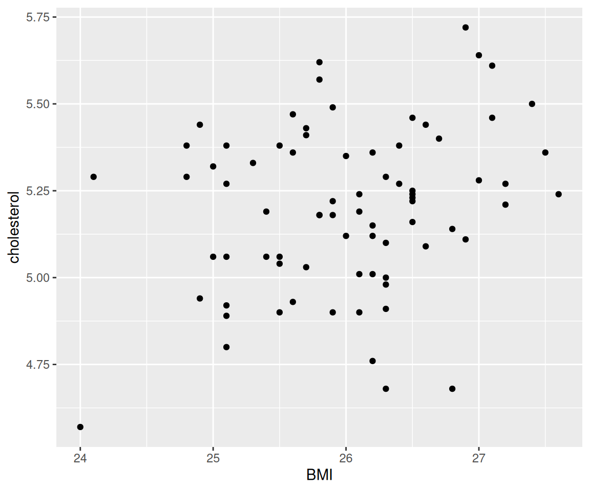 While this gets the job done, it doesn’t look very elegant. Let’s take a look what this looks like when we use the pipe operator
 %>%.
I hope you agree that this looks more intepretable, with each line corresponding to a step in the data processing. The pipe operator %>% is a binary operator that takes the object on its left-hand side and passes it as the first argument to the function on its right-hand side. This makes it easier to read the code from left to right, as if you are reading a book.
From now on, we will be extensively using the pipe operator %>% to make the code more readable.
8.1.4 Exercises
Using the
ahpdataset, create a new tibble namedmy_ahpthat contains all houses that are built before year 2000 (not including 2000), sold on or after year 2009, and with 2 or 3 bedrooms.Using the
gmdataset, create a new tibble namedmy_gmthat contains all countries in Asia and Africa withHDI_categorybeing “high” or “medium” in year 2006.
