1.3 Object Assignment
In the last section, you saw how R handles one-off calculations. To carry out a full analysis, though, you almost always need to preserve the output from one step so you can use it again later.
Consider the following three calculations, each of which repeats the expression exp(3) / log(20, 3) * 7.
(exp(3) / log(20, 3) * 7) + 3 #addition
(exp(3) / log(20, 3) * 7) - 3 #subtraction
(exp(3) / log(20, 3) * 7) / 3 #division
Typing the same expression three times invites typos and makes future edits painful. Object assignment lets you store that intermediate value once and reuse it wherever you need it.
1.3.1 What is an R Object?
Before we talk about assignment, we need to clarify what an object is. In R, everything you work with is an object: the number 5, the expression 1 + 2, and even the result of exp(3) / log(20, 3) * 7.
Running one of those expressions prints its value. In these simple examples each object has a single element, but objects can also hold multiple elements (for example, a vector of several numbers), each retaining its own value. You will soon learn how to create named objects and control what they store.
1.3.2 Assignment Operation with <-
With objects in mind, the next step is to learn how to create a named object. The basic pattern is name <- value: choose a descriptive name, place the assignment operator <- in the middle, and supply the value you want to store. Once the object exists, you can reuse the name in later expressions without retyping the original value. Here is the simplest possible example.
The expression has three parts: the object name (x_num), the assignment operator (<-, written with no space between < and -), and the value being stored (the number 5). Naming rules are covered in Section 1.3.3.
Keep the two characters of <- together. Although R also accepts =, we strongly recommend reserving = for function arguments (to be introduced in Section 2.1); mixing the two styles easily leads to confusing code.
Running the assignment prints nothing to the console (Figure 1.18), unlike 1 + 2 which displays 3. The object is created quietly in the background.
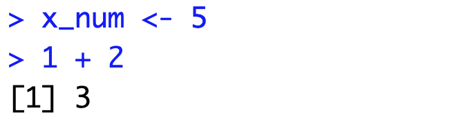
Figure 1.18: No output during the assignment operation.
To confirm the value stored in an object, run a line containing only its name. R prints the contents of the object to the console.
Great! The output 5 shows that the name x_num now stores the value 5. Anywhere you would have typed the literal number, you can now reference x_num instead.
Note that R object names are case-sensitive. For example, you defined x_num, but if you type X_num, the console returns an error because R treats those names as different objects.
You can also assign the result of an expression to a name. Let’s simplify the three expressions we showed at the beginning of this section. Each one shares the common term exp(3) / log(20, 3) * 7, so we will store that term in an object.
Now you have successfully created an object y_num that stores the numeric value 51.561191. Using the named object y_num, you can simplify the three calculations as follows.
During assignment, the expression on the right-hand side is evaluated first and only the resulting value is stored. Running y_num therefore returns the numeric result, not the text of the original expression.
Try the following examples to see a few more assignment patterns.
Clearly, object assignment greatly simplifies the code and avoids redundant typing.
1.3.3 Object Naming Rules
R is fairly flexible about object names, but three rules are non-negotiable. Practicing them early will save you from obscure bugs later.
a. Start with a letter or a single . (period)
If you start a name with ., the second character cannot be a number.
b. Use only letters, numbers, _ (underscore), or . (period)
A consistent style improves readability. We recommend all-lowercase names separated with underscores, such as this_is_name_6 or super_rich_88.
c. Avoid reserved keywords
Names such as TRUE, if, or function are reserved by R and cannot be reassigned. Attempting to do so results in an error, as shown below.
Some common reserved keywords that cannot be used as names are listed below.
| TRUE | else |
| FALSE | for |
| NA | while |
| Inf | break |
| NaN | next |
| function | repeat |
| if | return |
To get a complete list of reserved words, you can run the following code.
1.3.4 Review objects in environment
You can inspect your objects visually in the Environment pane, located in the top-right area of RStudio (panel 3 in Figure 1.4 from Section 1.1).
If you ran the earlier examples, you should now see objects such as x_num, y_num, and z_num1 listed in the Environment tab (Figure 1.19). Reserved keywords like TRUE never appear because R refuses to overwrite them.
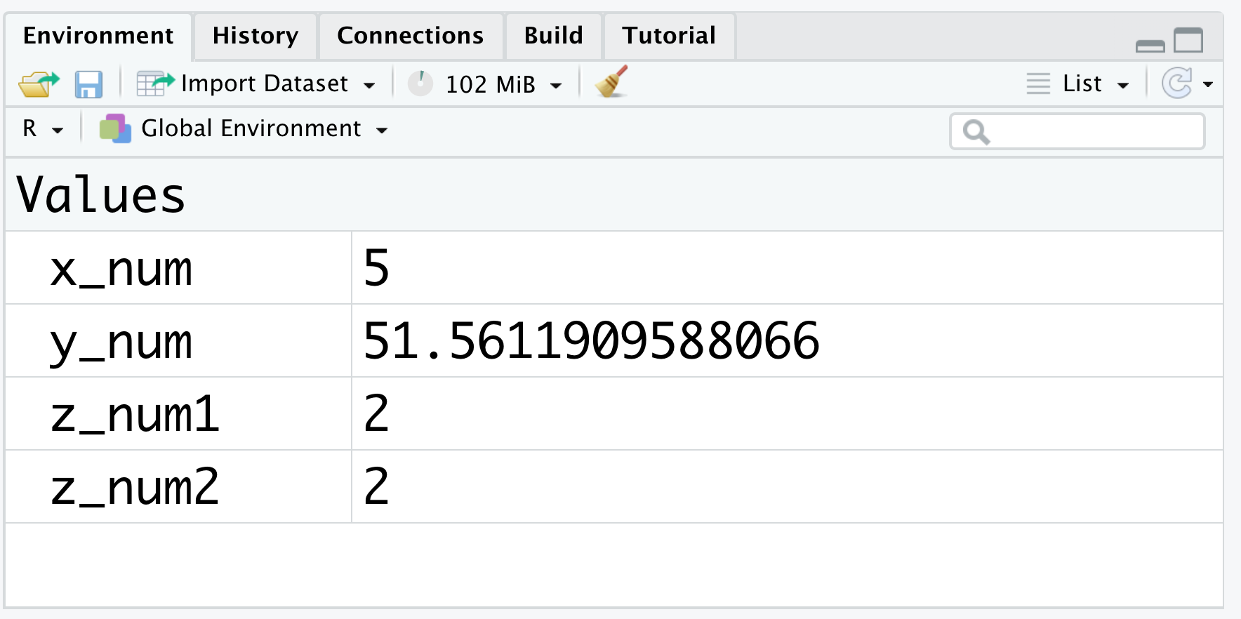
Figure 1.19: The environment (I)
From the screenshot above you can see that x_num currently stores the value 5. Let’s update it to 6 and observe what changes.
The Environment now shows x_num with value 6. Assigning a new value replaces the old one; R does not keep past values once you reassign the name.
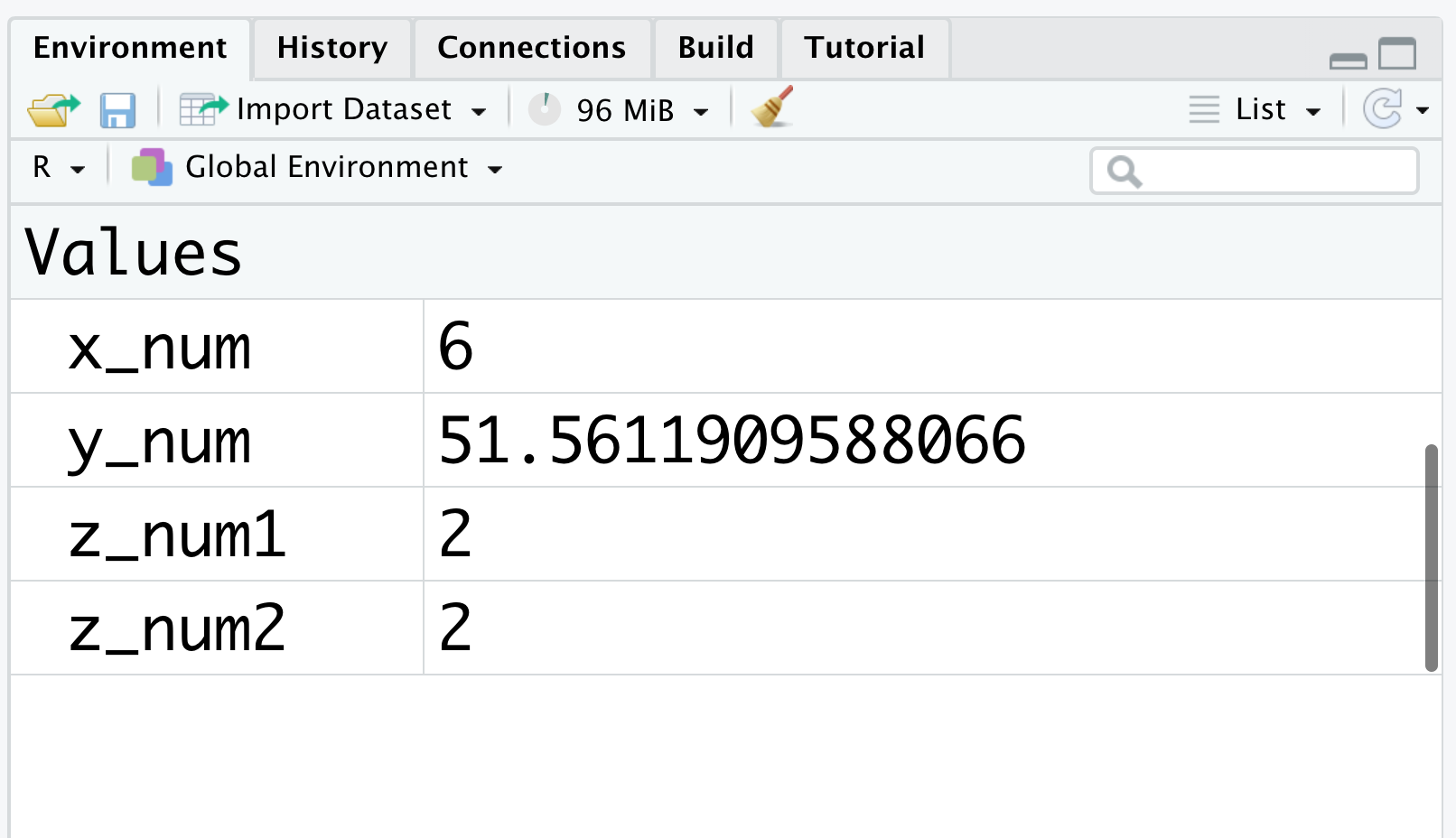
Figure 1.20: The environment (II)
Keep an eye on the Environment pane while you work to confirm objects contain what you expect. Only named objects appear there; unnamed results vanish as soon as they are printed.
You can also list the names programmatically with the built-in ls() function. The function returns a character vector, which means you can combine it with other functions (length(ls()), rm(list = ls()), and so on) when you want to audit or tidy your workspace from the console.
Everything shown in the Environment pane or returned by ls() lives in memory, ready for reuse in later code. Assigning important results to objects and removing ones you no longer need keep your workspace organized and your scripts reproducible.
1.3.5 Object types
So far we have assigned single numeric values to objects. In practice an object may contain many values at once, and those values do not have to be numeric: text strings, logical values, and dates all appear routinely in data analysis. The composition of values determines the object type.
| Type | Section |
|---|---|
| Atomic Vector | 2 |
| Matrix | 4.1 |
| Array | 4.2 |
| Data Frame | 4.3 |
| Tibble | 4.4 |
| List | 4.5 |
We will focus on atomic vectors in Chapters 2 and 3 and explore the remaining object types in Chapter 4.
Some object types look more intuitive than others, but the next two chapters walk through each in detail. Objects are the building blocks of R programming, so the time you invest in understanding them will pay off quickly.
