1.1 Installation of R, RStudio and R Packages
1.1.1 Download and Install
First, download R and RStudio using the links below. Select the installer that matches your operating system.
Download R: https://cloud.r-project.org/
Download RStudio: https://rstudio.com/products/rstudio/download/#download
RStudio is an Integrated Development Environment for R, which is powerful yet easy to use. It places the console, a syntax-highlighting editor, a workspace browser, and many other tools in a single window.
1.1.2 RStudio Interface
After opening RStudio for the first time, you may find that the font and button size is a bit small. Let’s see how to customize the appearance.
a. Customize appearance
On the RStudio menu bar, you can click Tools, and then click on Global Options as shown below.
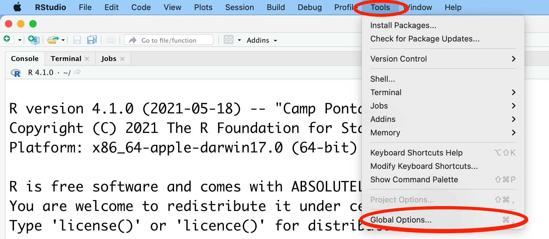
Figure 1.1: Global Options
Then, you will see a window popping up like Figure 1.2. After clicking on Appearance, you can see several drop-down menus including Zoom and Editor font size among other choices shown.
Zoom controls the overall scale for all elements in the RStudio interface, including the sizes of the menu, buttons, as well as fonts.
Editor font size controls the size of the font only in the code editor.
Once finishing customizing the appearance, you need to click on Apply to save the adjustments.
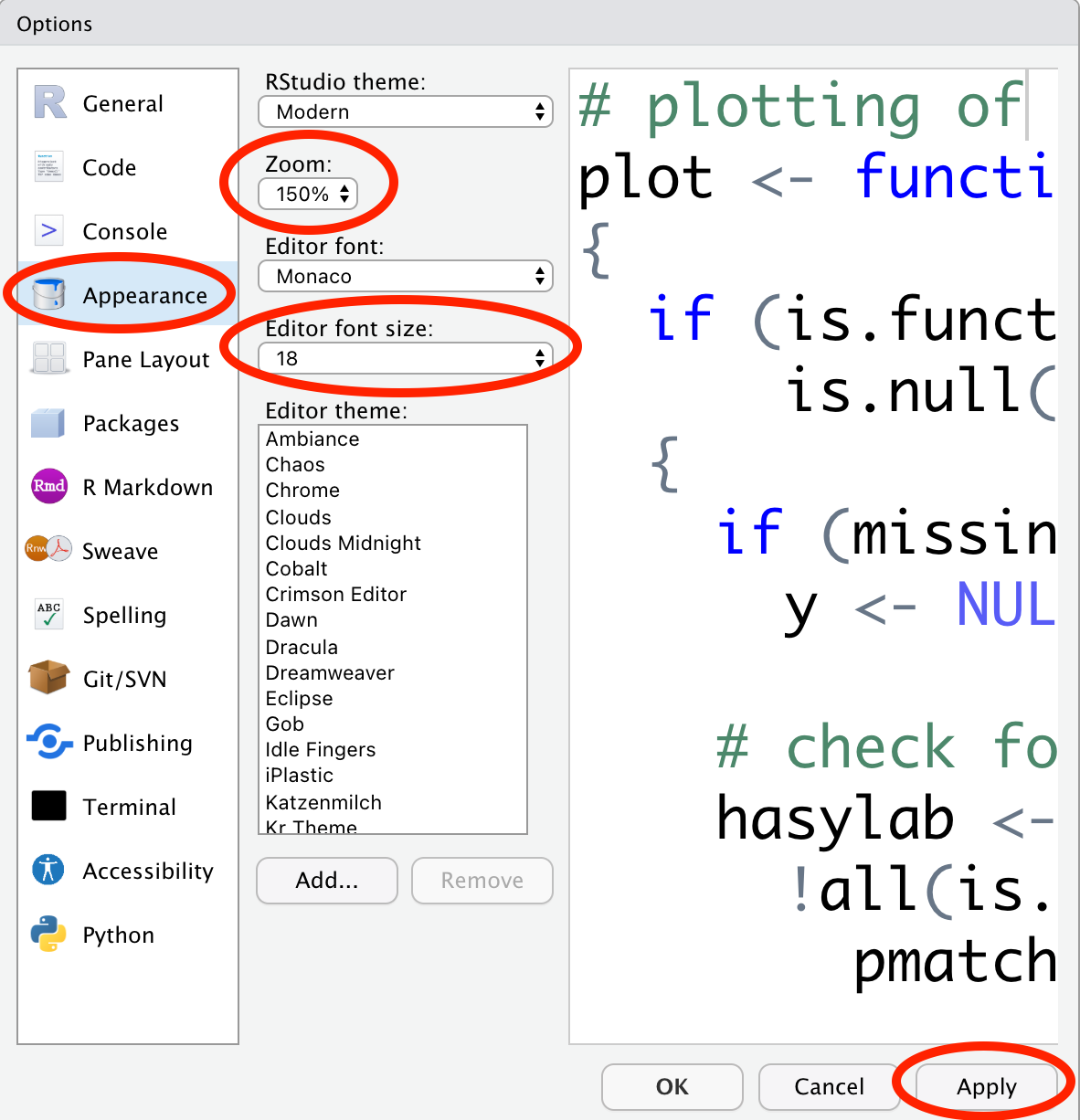
Figure 1.2: Zoom and Editor font size
Here, we change the Zoom to 150% and set the Editor font size to 18.
b. Four panels of RStudio
Although RStudio has four panels, some may be hidden initially (Figure 1.3).
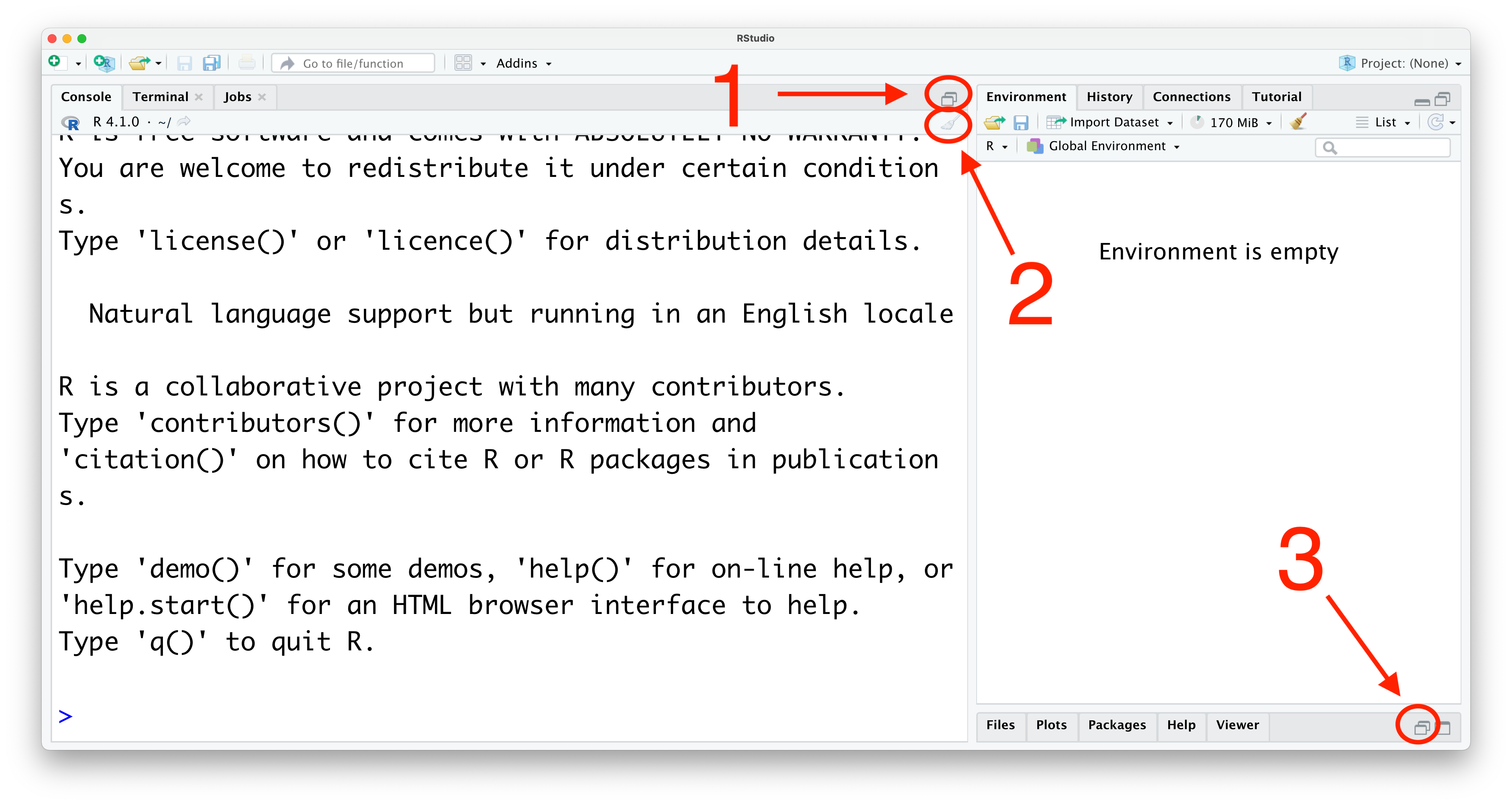
Figure 1.3: Unfold panels
In Figure 1.3, we have labeled three useful buttons as 1, 2, and 3. By clicking buttons 1 and 3, you can reveal the two hidden panels.
Note that you may see different panels hidden when you open RStudio for the first time, depending on the RStudio version. However, you can always reveal the hidden panels by clicking the corresponding buttons like Buttons 1 and 3 in Figure 1.3.
By clicking button 2, we can clear the content in the bottom left panel (Panel 2 in Figure 1.4) as shown in the following figure.
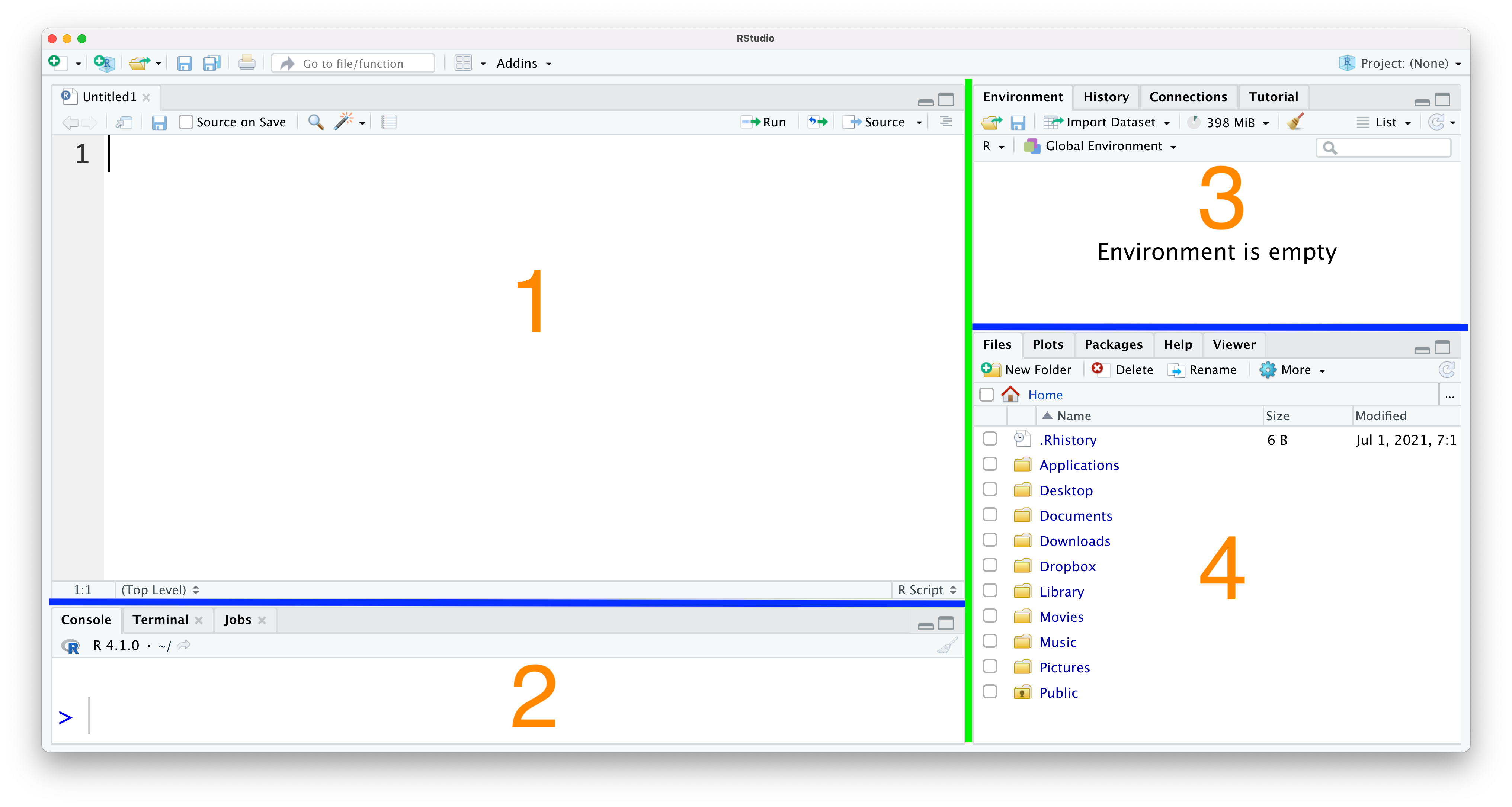
Figure 1.4: Four panels
Now, let’s take a close look at all four panels, which are labeled as 1-4 in Figure 1.4. You can change the size of each panel by dragging the two blue slides up or down and the green slide left or right.
Located to the left of the green line, Panels 1 and 2 together compose the Code Area. We will introduce them in the following parts of this section.
Located to the right of the green line, Panels 3 and 4 together make up the R Support Area. We will introduce these two panels in later sections.
c. Console
Firstly, we will introduce panel 2 in Figure 1.4, which is usually called the Console. The console window is the place for you to type in codes (i.e. the things you want R to do) and you will get the results immediately once you run the codes.
By clicking the mouse on the line after the > symbol, you can see a blinking cursor, indicating that R is ready to accept codes. Let’s type 1 + 2 and press Return (on Mac) or Enter (on Windows).
It is a good habit to add spaces around an operator to increase the readability of the code.
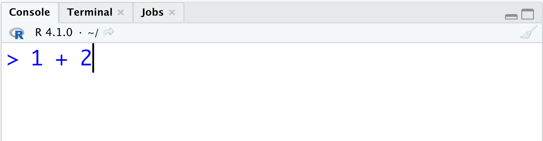
Figure 1.5: Writing code in the console
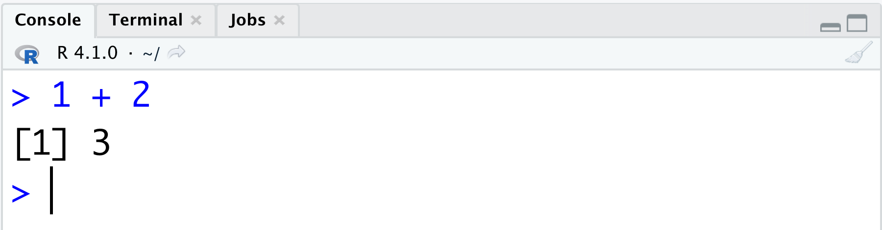
Figure 1.6: R code(2)
Hooray! You have successfully run the first piece of R code and gotten the correct answer 3. Note that the blinking cursor now appears on the next line, ready to accept a new line of code.
The curious you may found that there is a [1] showing before the result 3. In fact, the [1] is an index indicator, showing the next element has an index of 1 in this particular object. We will revisit this point when we introduce vectors in Chapter 2.
Although the console may work well for some quick calculations, you need to resort to panel 1 in Figure 1.4 (known as the Editor) to save our work and run multiple lines of code at once.
d. Editor
The Editor panel is the go-to place to write complicated R codes, which you can save as R files for repeated use in the future. Several kinds of files are available in RStudio. In particular, R script and R Markdown are the two most common file formats. We will start with R script since it is the simplest format. In Chapter 1.4, we will introduce R Markdown in detail.
In the editor panel, you may notice that RStudio has created a file by default (Figure 1.7). The default file RStudio provided is R script.
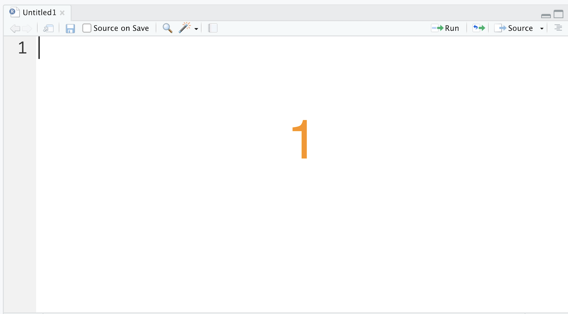
Figure 1.7: R script
Next, we will introduce how to run codes in scripts. Let’s go to the editor and type 1 + 2. To run this line of code, you can select this line of code and click the Run button. The keyboard shortcut of running this line of code is Cmd+Return on Mac or Ctrl+Enter on Windows. RStudio will then send the line of code to the console and execute the code.
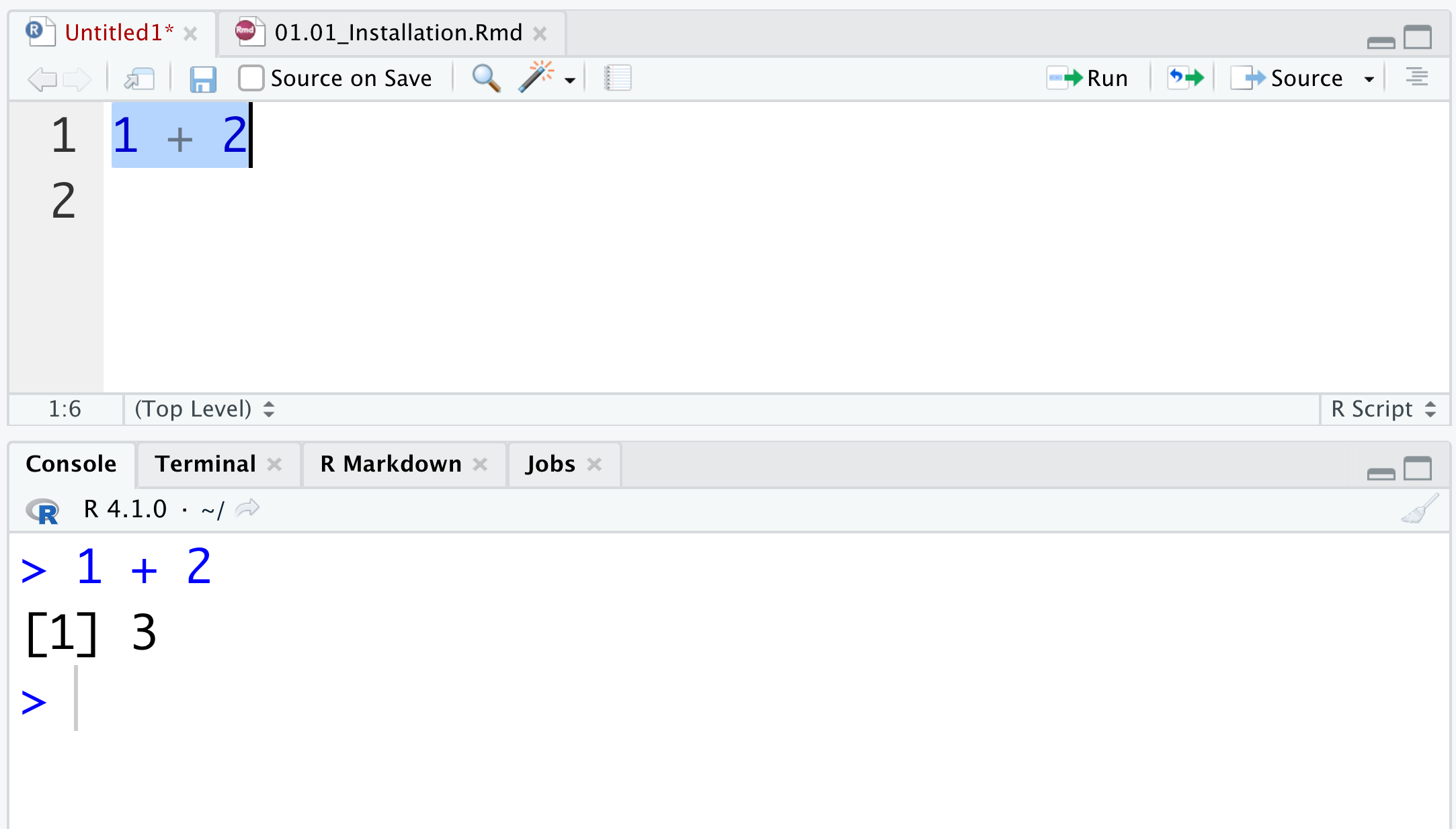
Figure 1.8: Run codes in script (I)
You can also run multiple lines of code by selecting the corresponding lines and clicking the Run button or using the keyboard shortcut. (Figure 1.9)
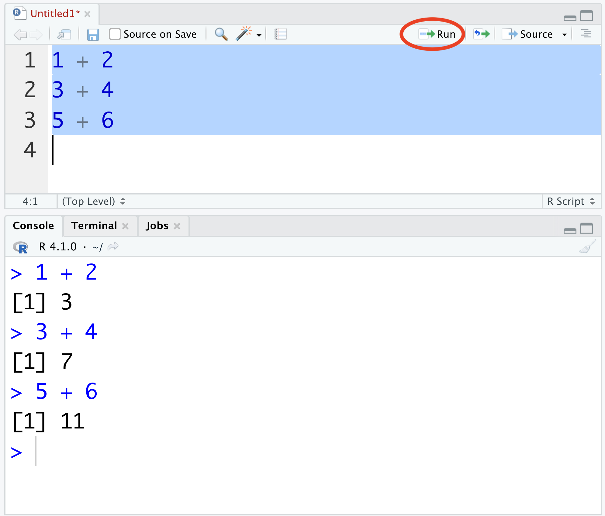
Figure 1.9: Run codes in script (II)
Here, three lines of codes are selected. After running these three lines of code together, you can see that the console executes all three lines of code and you will get the corresponding outputs one by one.
To save your work for later use, you can click the Save button as shown in Figure 1.10. The keyboard shortcut of saving files is Cmd+S on Mac or Ctrl+S on Windows.
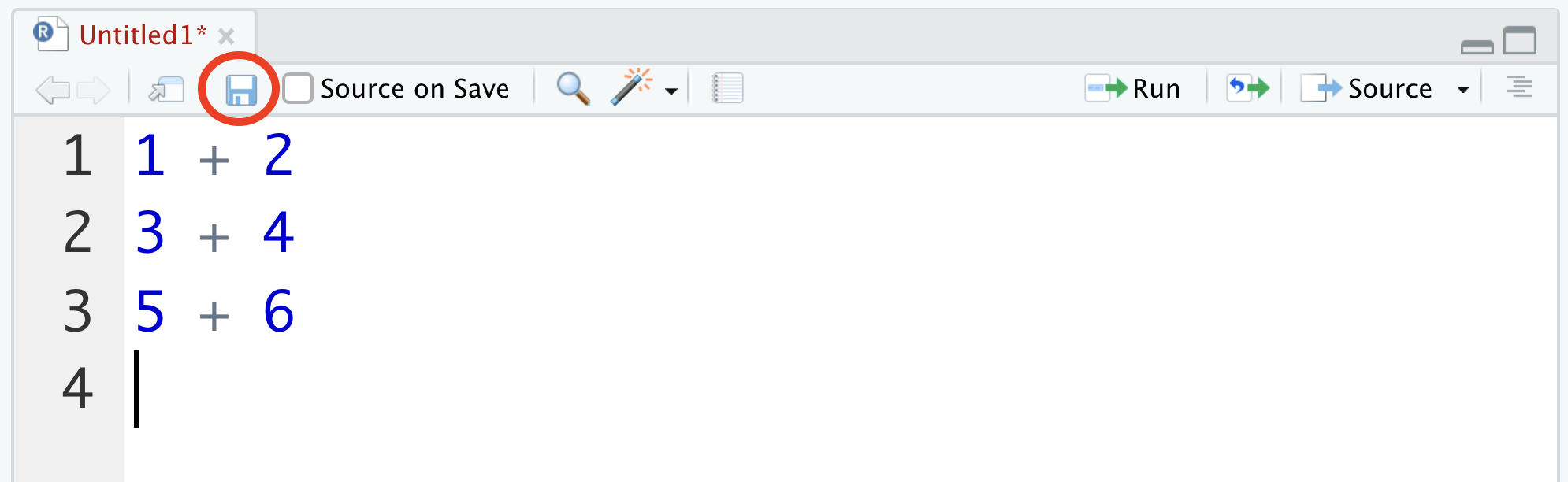
Figure 1.10: Save (I)
Then you would see a pop-up file dialog box, asking you for a file name and location to save it to. Let’s call it lesson1.1 here.
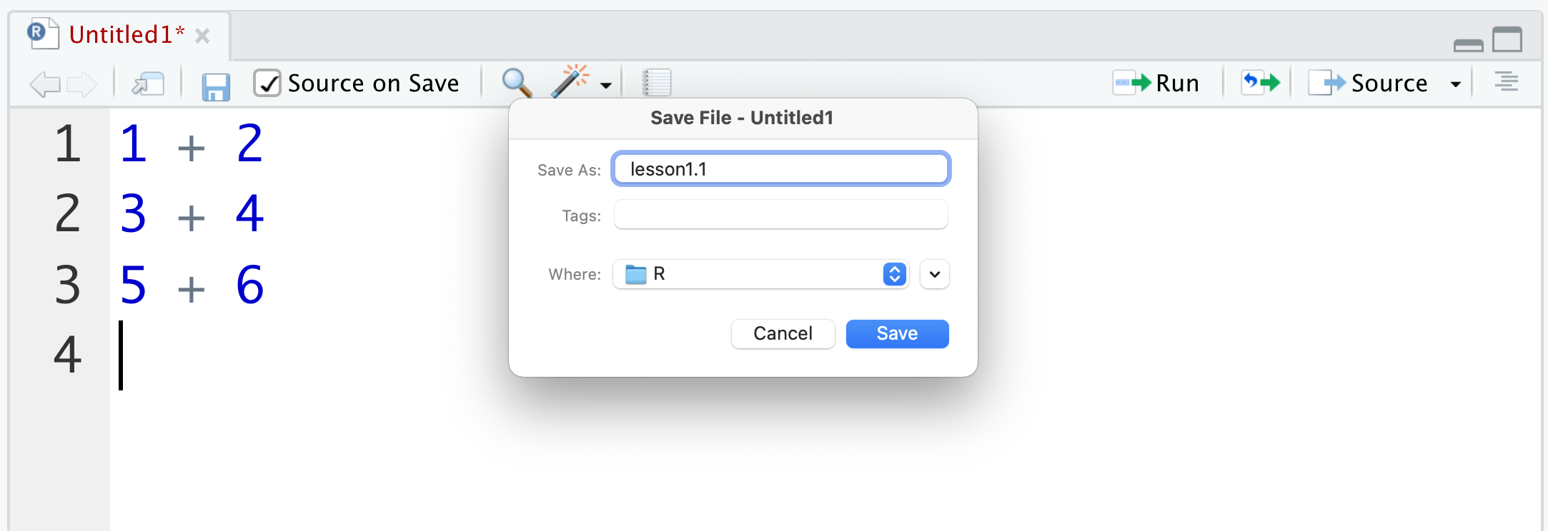
Figure 1.11: Save (II)
After saving the file successfully, you can confirm the name of the R script on the top.
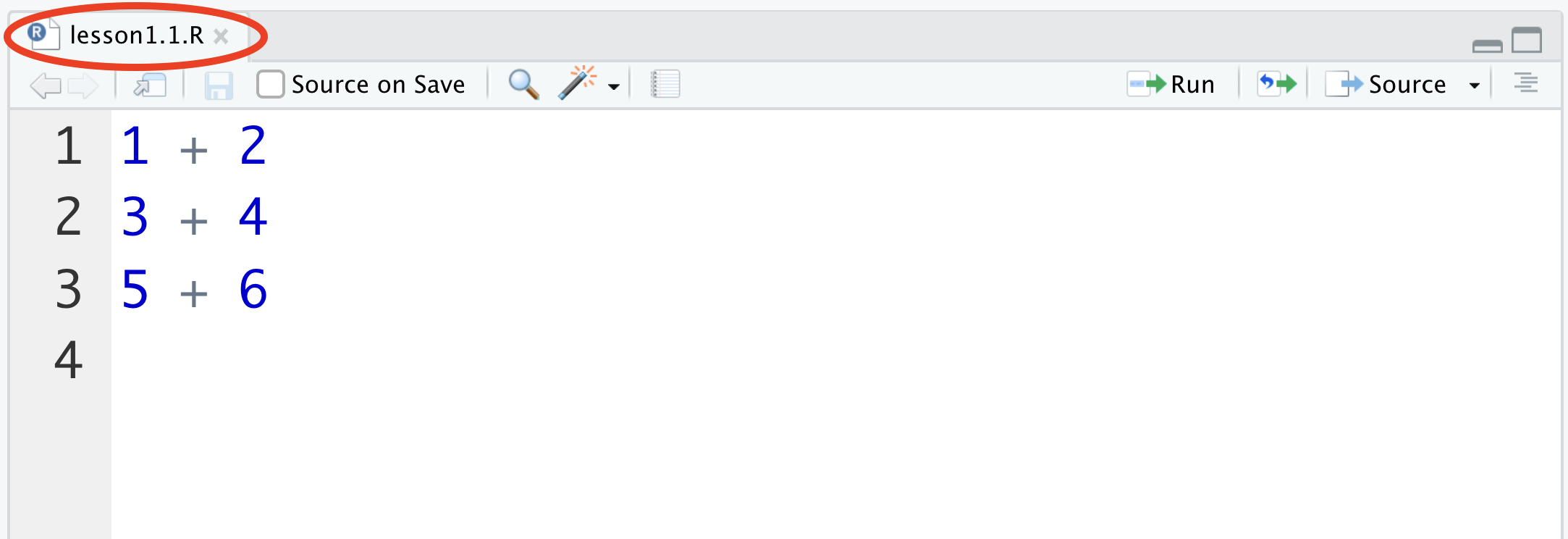
Figure 1.12: Save (III)
Now, when you close this script and open it again, you would directly see the previous three lines of codes.
Lastly, if you want to create a new R script, you can click the + button on the menu, then select R Script. Note that there are quite a few other options including R Markdown, which will be introduced in Chapter 1.4.
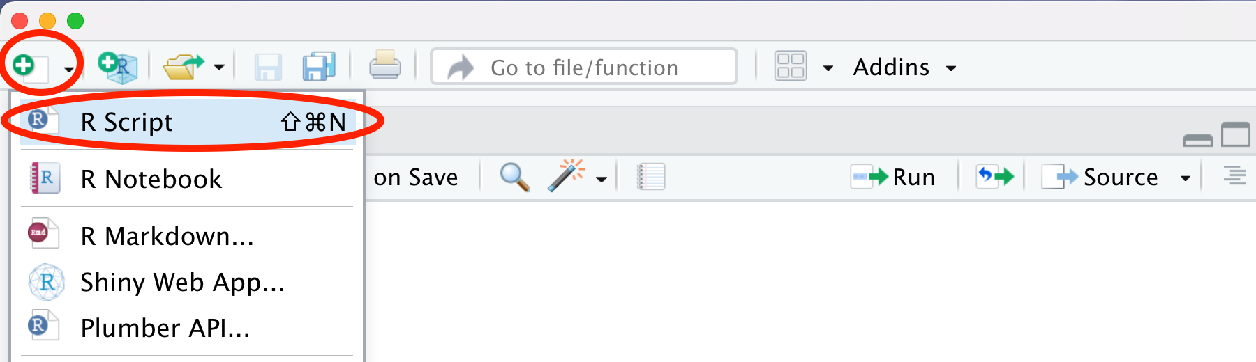
Figure 1.13: create a new script (I)
Consequently, you will see a new file created.
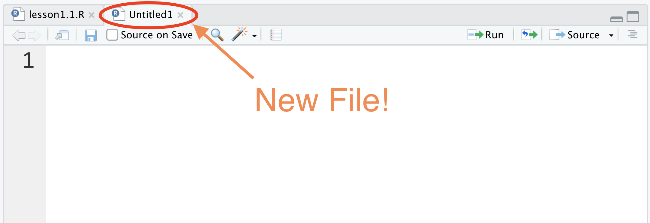
Figure 1.14: create a new script (II)
1.1.3 Install and load R packages
Now, you have had a basic understanding of RStudio, it is time to meet R packages, which greatly extend the capabilities of base R. There are a large number of publicly available R packages. As of July 2021, there are more than 17K R packages on Comprehensive R Archive Network (CRAN), with many others located in Bioconductor, GitHub, and other repositories.
To install an R package, you need to use a built-in R function, which is install.packages(). A function takes in arguments (inputs) and performs a specific task accordingly. After the function name, we always need to put a pair of parentheses with the arguments inside.
While there are many built-in R functions, R packages usually contain many useful functions as well, and we can also write our own functions, which will be introduced in Chapter 13.
With install.packages(), the argument is the package name with a pair of quotation marks around it. The task it performs is installing the specific package into R. Here, you will install the companion package for this book, named r02pro, a.k.a. R Zero to Pro. The r02pro package contains several data sets that will be used throughout the book.
If you miss the right parenthesis, R will return a plus in the next line (as shown in Figure 1.15), waiting for more input to complete the command. If this happens, you can either enter the right parenthesis, or press ESC to escape this command. When you see a blinking cursor after the > symbol, you can write new codes again.
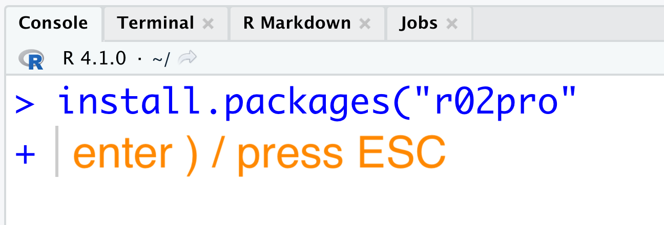
Figure 1.15: Miss the right parenthesis
After a package is installed, you still need to load it into R before using it. To load a package, you can use the library() function with the package name as its argument. Here, quotation marks are not necessary.
Note that once a package is installed, you don’t need to install it again on the same machine. However, when starting a new R session, you would need to load the package again.
