11.4 Multivariate Normal Distribution
In this section, we introduce how to work with multivariate normal distribution in R.
First, let’s review the definition of a multivariate normal distribution. Suppose a \(p\)-dimensional random vector \({\bf x} \sim N({\bf \mu}, {\bf \Sigma})\), where \({\bf \mu}\) is the mean vector and \({\bf \Sigma}\) is the covariance matrix. We have \[ f({\bf x}) = \frac{1}{(2\pi)^{p/2}\sqrt{|{\bf \Sigma}|}}\exp\left[-\frac{1}{2}({\bf x}-{\bf\mu})^T{\bf \Sigma}^{-1}({\bf x}-{\bf\mu})\right]. \]
11.4.1 Generate Multivariate Normal Distribution
To randomly generate \({\bf x} \sim N({\bf \mu}, {\bf \Sigma})\), you can use the mvrnorm(n = 1, mu, Sigma) function in the MASS package, which is pre-loaded in the base R. The function mvnorm() takes three arguments.
n: targeted sample sizemu: mean vectorSigma: covariance matrix
Let’s take a look at an example where the distribution is \(\bf\mu = (1, 2)^T\) and \[{\bf \Sigma} = \left[\begin{matrix} 1&0.8\\ 0.8&1 \end{matrix}\right]\]
library(MASS)
#>
#> Attaching package: 'MASS'
#> The following object is masked from 'package:plotly':
#>
#>     select
#> The following object is masked from 'package:dplyr':
#>
#>     select
set.seed(87)
n <- 1000
mu <- c(1, 2)
Sigma <- matrix(c(1, 0.8, 0.8, 1), 2, 2)
x <- mvrnorm(n, mu, Sigma)
head(x)
#>              [,1]        [,2]
#> [1,] -1.002876112 -0.06259489
#> [2,] -0.843956459  0.57515106
#> [3,] -0.158140872 -0.39338951
#> [4,] -0.004390677  1.26823724
#> [5,]  2.483115985  3.99971514
#> [6,]  0.526159176  2.27572849
x contains \(n=1,000\) two-dimensional normal distributed variable, where each row represents one observation. Let’s try to visualize the data using a scatterplot.
normal_data <- as.data.frame(x)
colnames(normal_data) <- c("X1", "X2")

library(ggplot2)
# Visualize using ggplot
ggplot(normal_data, aes(x = X1, y = X2)) +
  geom_point(color = "blue", alpha = 0.6) +
  labs(title = "Scatterplot of Multivariate Normal Data",
       x = "X1",
       y = "X2") +
  theme_minimal()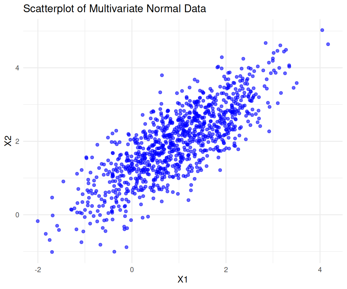
11.4.2 Properties of Multivariate Normal Distribution
- Marginal Distributions:
- Each component of \({\bf x}\) follows a univariate normal distribution.
- Linear Combinations:
- Any linear combination of the components of \({\bf x}\) is also normally distributed.
- Independence:
- Two components of \({\bf x}\) are independent if and only if their covariance is zero.
Let’s use visualizations to verify the properties of the multivariate normal distribution.
# Marginals visualization using ggplot
ggplot(normal_data, aes(x = X1)) +
  geom_histogram(bins = 30, fill = "lightblue", color = "black", alpha = 0.7) +
  labs(title = "Histogram of X1", x = "X1", y = "Frequency") +
  theme_minimal()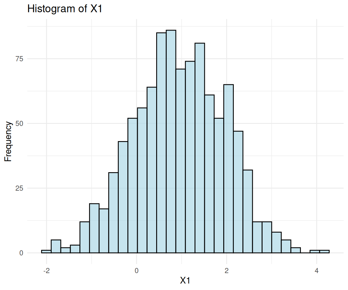
ggplot(normal_data, aes(x = X2)) +
  geom_histogram(bins = 30, fill = "lightgreen", color = "black", alpha = 0.7) +
  labs(title = "Histogram of X2", x = "X2", y = "Frequency") +
  theme_minimal()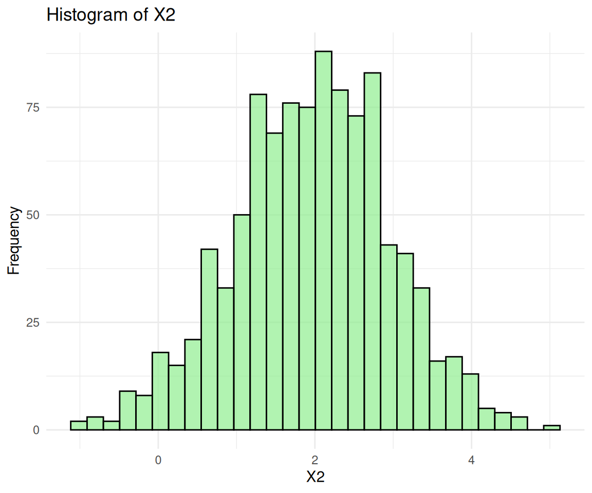
# Linear combination visualization
linear_combination <- 0.5 * normal_data$X1 + 0.5 * normal_data$X2
ggplot(data.frame(LinearCombination = linear_combination), aes(x = LinearCombination)) +
  geom_histogram(bins = 30, fill = "pink", color = "black", alpha = 0.7) +
  labs(title = "Histogram of Linear Combination",
       x = "Linear Combination",
       y = "Frequency") +
  theme_minimal()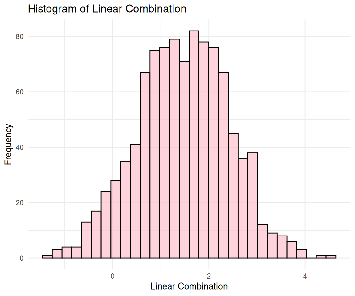
11.4.3 Sample Mean and Sample Covariance Matrix
In practical applications, we usually have a set of observations and would like to get a sample estimate of the parameters \({\bf \mu}\) and \({\bf \Sigma}\).
For the \({\bf \mu}\), you can directly use the sample mean as the estimate which is unbiased. \[\hat {\bf\mu} = [\hat\mu_j],\] where \[\hat\mu_j = \frac{1}{n}\sum_{i=1}^nx_{ij}.\]
To estimate \({\bf\Sigma}\), we will use the sample covariance matrix estimate: \[\hat{\bf \Sigma} = [\hat\Sigma_{jk}],\] where \[\hat\Sigma_{jk} = \frac{1}{n-1}\sum_{i=1}^n(x_{ij}-\hat\mu_j)(x_{ik}-\hat\mu_k).\]
To compute this matrix, we can use the function cov() on the matrix x.
sigma_hat <- cov(x)
sigma_hat
#>           [,1]      [,2]
#> [1,] 1.0042256 0.8036966
#> [2,] 0.8036966 0.9964596
1/(n-1)*sum((x[,1]-mu_hat[1])*(x[,2]-mu_hat[2])) #compute \hat\Sigma_{12} by formula
#> [1] 0.8036966
For cov() function, in addition to computing the sample covariance matrix, you can also use it to compute the covariance among two vectors \(y\) and \(z\).
\[cov(y, z) = \frac{1}{n-1}\sum_{i=1}^n(y_{i}-\bar y)(z_i-\bar z).\]
Let’s try to compute the covariance between the first and second column of \(x\).
You can see that this is exactly the same as \(\hat\Sigma_{12}\).
11.4.4 Sample Correlation Matrix
Another useful measure is the sample correlation matrix. It is defined as \[\widehat{corr}(x) = [\widehat{corr}(x)_{jk}],\] where \[\widehat{corr}(x)_{jk} = \frac{\hat\Sigma_{jk}} {\sqrt{\hat\Sigma_{jj}\hat\Sigma_{kk}}}. \]
You can use cor() on the matrix x to get its sample correlation matrix.
cor(x)
#>           [,1]      [,2]
#> [1,] 1.0000000 0.8034274
#> [2,] 0.8034274 1.0000000
sigma_hat[1,2] / sqrt(sigma_hat[1, 1] * sigma_hat[2, 2]) #verify the [1,2] element
#> [1] 0.8034274
Similar to the cov() function, you can also us the cor() function to compute the sample correlation between two vectors.
You can see that the sample correlation matrix include all the pairwise sample correlations between any of the two columns.
11.4.5 Exercises
- Generate 500 observations from a bivariate normal distribution with:
- Mean vector \({\bf \mu} = (3, 5)^T\)
- Covariance matrix \({\bf \Sigma} = \begin{bmatrix} 2 & 0.5 \\ 0.5 & 1 \end{bmatrix}\).
- Visualize the data using a scatterplot with
ggplot2.
- For the above data:
- Plot the histograms of each marginal distribution using
ggplot2. - Compute and interpret the covariance and correlation.
- Plot the histograms of each marginal distribution using
- Generate 1000 observations from a 3-dimensional normal distribution with:
- \({\bf \mu} = (1, -1, 3)^T\)
- \({\bf \Sigma} = \begin{bmatrix} 1 & 0.3 & 0.2 \\ 0.3 & 1 & 0.4 \\ 0.2 & 0.4 & 1 \end{bmatrix}\).
- Compute the pairwise sample correlations between dimensions.
