2.1 Introduction to Numeric Vectors
We will start off this chapter by learning numeric vectors. Numeric vectors are perhaps the most commonly used member of the atomic vector family, where all elements are of the same type.
2.1.1 Creation and class
A numeric vector is an atomic vector containing only numbers. For example, 6 is a numeric vector with one element of value 6.
By assigning the value 6 to the name x1, you can create a numeric vector x1 with value 6. Then, you can refer to x1 in subsequent calculations. For any vector, you can use the length() function to check the number of elements it contains.
6                         #a numeric vector
#> [1] 6
x1 <- 6                   #x1 is now another numeric vector
x1                        #check the value of x1
#> [1] 6
length(6)                 #length of 6
#> [1] 1
length(x1)                #length of x1
#> [1] 1
From the output, you can see that 6 is a numeric vector with length 1, and x1 is also a numeric vector with length 1. The value of x1 is 6, which is the same as the value of 6.
Moving on, you may wonder, can a numeric vector contain more than one values? The answer is a big YES! In R, you can use the c() function (c is short for combine) to combine several elements into one single numeric vector.
c(1, 3, 3, 5, 5)          #combine elements
#> [1] 1 3 3 5 5
y1 <- c(1, 3, 3, 5, 5)    #y1 is a numeric vector of length 5
y1                        #check the value of y1
#> [1] 1 3 3 5 5
length(y1)                #length of y1
#> [1] 5
In this example, you have created a numeric vector y1 with five elements: 1, 3, 3, 5, and 5. Notice that the c() function can take multiple arguments separated by commas. The length of y1 is 5 since it contains five elements.
When you assign multiple values to a vector, R preserves the exact order of elements as you specify. If you create two numeric vectors containing the same numbers but in different orders, they are considered two distinct vectors because the order of elements matters in R.
For example:
Although y2 and y3 contain the same set of numbers, their element order is different, making them different vectors.
In addition to using numbers inside the c() function, you can also use numeric vectors as arguments to create a longer vector. The new, longer vector will combine the input numeric vectors in the given order.
c(x1, y1)          #combine several numeric vectors
#> [1] 6 1 3 3 5 5
z1 <- c(x1, y1)
z1
#> [1] 6 1 3 3 5 5
length(z1)
#> [1] 6
Since x1 contains one numeric value and y1 contains five numeric values, z1 is a numeric vector of length 6 after combination.
For any vector, you can use the function class() to check its class. A class can be viewed as a “type,” providing a description about the vector and determining what functions can be applied to it.
From the results, you can see that x1, y1, and z1 are all numeric, which is the reason why they are called numeric vectors.
As introduced in Section 1.3, you can check the named objects via the environment panel as shown in Figure 2.1.
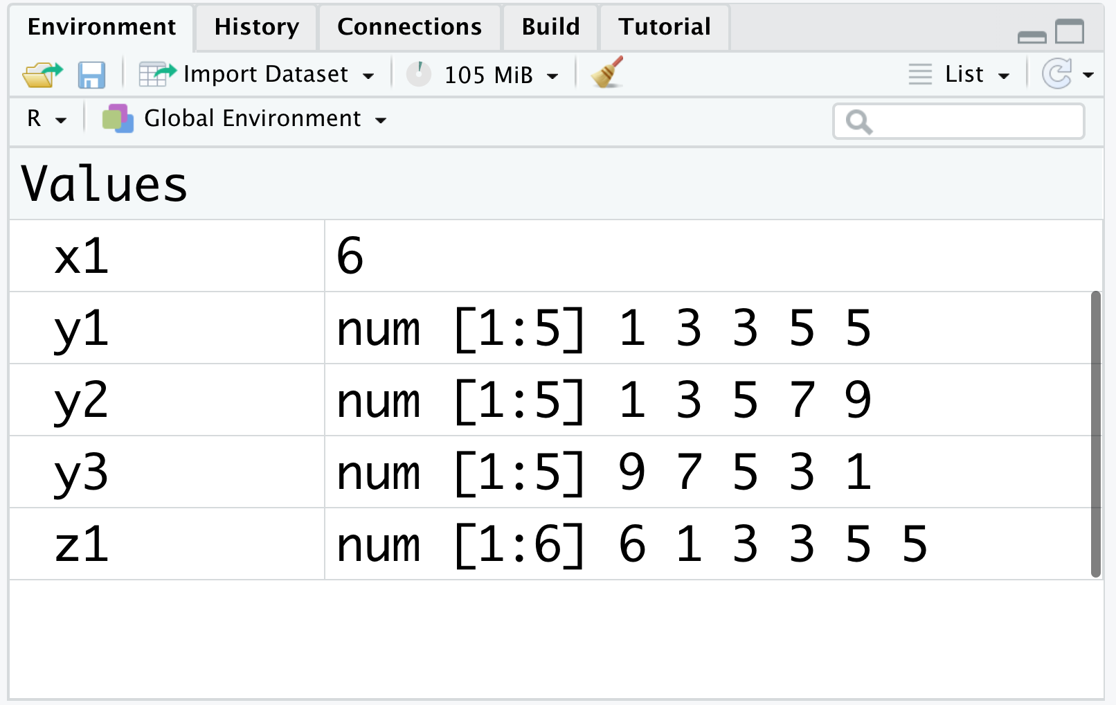
Figure 2.1: The environment (I)
We can see that the environment panel has two columns, with the first column showing the list of object names and the second column showing the corresponding information for each object. The information includes the vector type (here num is short for numeric), the vector length, and the value(s) of the vector. Note that if the vector is of length 1 (for example x1), the environment will not show the type or the length.
In the last section, we have introduced how to change the value of an object by reassigning it. Similarly, you can also assign a new value, or new values, to z1.
Now, you can see that z1 contains 3 numeric values, so z1 is a numeric vector of length 3.
As expected, you can also view the newly assigned values of z1 in the environment panel, as shown in Figure 2.2.
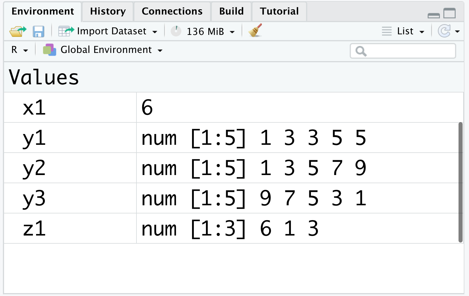
Figure 2.2: The environment (II)
Finally, you can use the vector(mode, length) function to create a vector of certain mode and length.
2.1.2 Operations and recycling rule
Since numeric vectors are purely made of numbers, you can do arithmetic operations between them, just like the fancy calculator in Section 1.2. If two or more vectors are of the same length, the operation is done element-wisely. In other words, R will perform the operation between elements in the same index of different vectors. First, let’s create another vector x2 of length 1 and compute the sum of x1 and x2. Also recall that we’ve previously created a length-1 numeric vector x1 with value 6.
The result is a length-1 numeric vector with value 9, which is the sum of 6 and 3.
If you assign this operation to a name, you will create a new numeric vector with the result of the operation as the value.
Here, s1 is a length-1 numeric vector with value 9.
Similarly, you can create another vector y2 of the same length as vector y1. Then, you can do operations between y1 and y2.
The result is yet another length-5 vector. To check the calculation was indeed done element-wisely, you can verify that the value of the first element is \(1 * 2 = 2\), and value of the second element is \(3 * 4 = 12\), etc.
You can also store the result of multiplication for future use by assigning it to a name.
To have the calculation done element-wisely, R requires two or more vectors to have the same length. However, there is an important recycling rule in R, which is quite useful and enables us to write simpler code.
What is recycling? When you perform an arithmetic operation between two vectors of different lengths, R will repeat (recycle) the elements of the shorter vector from the beginning until it matches the length of the longer one. Only then does R perform the element-wise operation.
The most common use of recycling is an operation between a vector and a scalar (a length-1 vector). Let’s see an example.
Here, y1 is a length-5 vector (c(1, 3, 5, 2, 4)) and x1 is a length-1 vector (6). R internally recycles x1 into c(6, 6, 6, 6, 6) and then performs element-wise addition:
    y1:    1    3    5    2    4
    x1:    6    6    6    6    6   <- recycled from length 1 to length 5
  ----  ----  ----  ----  ----  ----
  sum:    7    9   11    8   10
So the output is a length-5 numeric vector where each element of y1 has been increased by 6.
By now you have created several objects, and you may find that objects will not be saved in R if you don’t assign their values to names, for example, the results of y1 + x1 is not shown in the environment.
The followings are a few additional examples you can try.
In an operation between two vectors where the length of the longer vector is not a multiple of the length of the shorter vector, R will still recycle the shorter vector, but it will give a warning. For example, if you try to do y1 + c(1, 2), you will get a warning message saying that the longer object length is not a multiple of the shorter object length.
2.1.3 Storage types (doubles and integers)
Now, it is time to learn how numeric vectors are stored in R. To find the internal storage type of an R object, you can use the typeof() function.
You can see that the internal storage type of my_num is double, meaning that my_num is stored as a double precision numeric value. In fact, R stores numeric vectors as double precision vectors by default. Let’s see another example,
Different from my_num which contains a non-integer (1.5), all elements in my_dbl are integers. However, the storage type of my_dbl is still double, same as my_num. When all values of a numeric vector are integers (such as my_dbl), you can store it as an integer vector, which is also a numeric vector. To do this, you only need to put an “L” after each integer in the vector. Let’s create an integer vector and check its storage type as well as its class.
You can see that the internal storage type of my_int is indeed of integer type, with the class of it being integer as well. It is also worth noting that the displaying value of my_dbl and my_int are the same.
You can also check the vector type and values in the environment. (as shown in Figure 2.3)
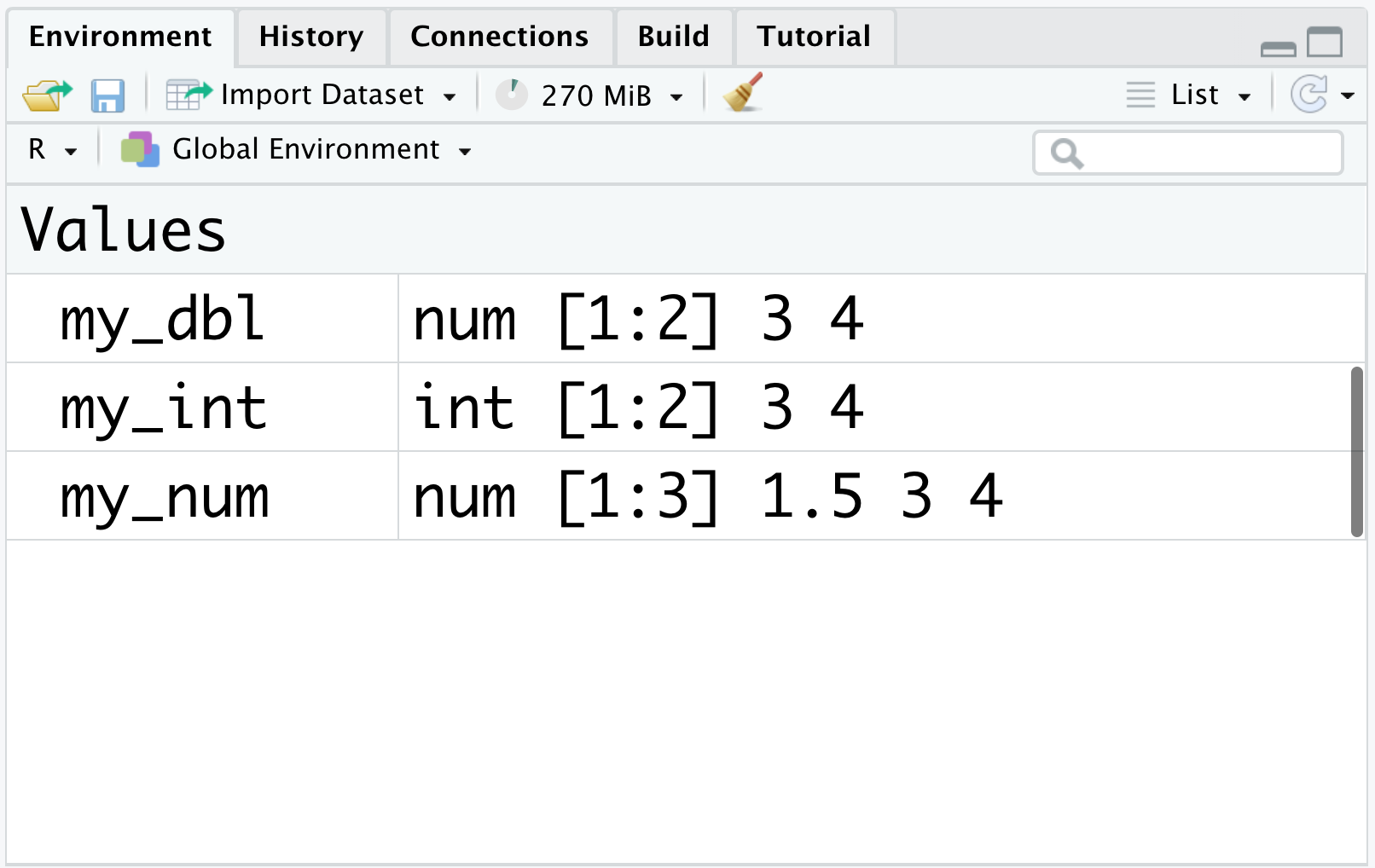
Figure 2.3: Different storage types
From the above image, you can see that the values of my_int are still 3 and 4, which are the same as those of my_dbl. The difference between these two vectors is that my_int is an integer vector since its internal storage type is integer, and such a storage type offers great memory savings compared to doubles.
Note that a numeric vector’s internal storage type is consistent for all its elements. Say if you assign multiple numeric values to an object, even when you assign an “L” to most values, as long as the object obtains at least one decimal value, the vector will be stored in R as double. This rule also implies that any numeric vector containing at least one decimal value cannot be transformed to an integer vector.
Moreover, as you can see by running the code below, whenever you put an “L” after an decimal value, you will get the warning and the storage type will remain double.
In conclusion, all the numeric vectors will be stored as double by default. If all values in a numeric vector are integers, you can convert this numeric vector into an integer vector, and the storage type of this vector will be integer, which leads to memory savings compared to doubles.
Despite the differences between integers and doubles, you can usually ignore their differences unless you are working on a very big data set. R will automatically convert objects between integers and doubles when necessary.
2.1.4 Printing
Now, you have learned numeric vectors along with their possible storage types. In this part, let’s discuss how you can customize the output digit of a number via printing. Let’s start with pi (\(\pi\)), which is a mathematical constant you may be familiar with. pi is also an internal numeric vector available for use in R, meaning that it will appear in the environment panel without requiring you to assign it to a name.
As you can see from the output, R prints out 7 significant digits by default, though in fact we need infinitely many digits to faithfully represent pi. To print out an object with a customized significant digit number, you can use the print() function that contains useful argument called digits, which controls the number of significant digits to be printed. Let’s see the following examples.
You can try the following examples.
print(pi, digits = 20)          #print pi for 20 significant digits
#> [1] 3.141592653589793116
print(pi, digits = 4)           #print pi for 4 significant digits
#> [1] 3.142
Note that the round() function also has an argument digits, which has a different meaning, representing the number of digits after the decimal point.
You may be wondering what happens if digits is larger than the number of the actual significant digits of a number. Let’s try the following example.
Clearly, the print() function will print out at most the significant digits of the number.
When you print a vector with more than one element, the same number of decimal places is printed for all elements. In this case, the digits parameter represents the minimum number of significant digits, and that at least one element will be encoded with that minimum number.
print(c(pi, exp(1), log(2)), digits = 4)
#> [1] 3.1416 2.7183 0.6931
print(c(pi, exp(1), log(2), exp(-5)), digits = 4)
#> [1] 3.141593 2.718282 0.693147 0.006738
print(c(20000, 1.2, 2.34), digits = 3)
#> [1] 20000.00     1.20     2.34
As you can imagine, the print() function will be very useful in creating tables that look more streamlined.
2.1.5 Exercises
Write R codes to complete the following tasks.
Create a numeric vector named
vec_1with values \((2, 4, 6, 8)\), get its length, find out its class, and get its storage type.For the numeric vector
vec_2 <- c(1, 3, 7, 10), get the value of the 3rd element, multiple the 3rd element by 5, and verify the change.Create a vector
vec_3where each element is twice the corresponding element invec_1minus half the corresponding element invec_2.Create an integer vector
int_1that contains integers \((2, 4, 6, 8)\). Check its class and storage type.Print out the vector \((\pi, \pi^2, \pi^3)\) with 5 significant digits.
