11.1 Normal Distribution
First, let’s review the definition of normal distribution, which is also called Gaussian distribution. If \(X\sim N(\mu, \sigma^2)\), we say \(X\) is a random variable following a normal distribution with mean \(\mu\) and variance \(\sigma^2\).
The normal distribution plays a central role in statistics due to the Central Limit Theorem, which states that the sum of many independent and identically distributed random variables tends to follow a normal distribution, regardless of their original distribution. It appears frequently in natural and social sciences as a model for measurement errors, test scores, heights, etc.
In the following table, we list the four useful functions for normal distribution, and they will be introduced in the subsequent four parts, respectively.
| Code | Name | Section |
|---|---|---|
dnorm(x, mean, sd) |
probability density function (PDF) | 11.1.1 |
pnorm(q, mean, sd) |
cumulative distribution function (CDF) | 11.1.2 |
qnorm(p, mean, sd) |
quantile function (QF) | 11.1.4 |
rnorm(n, mean, sd) |
random number generator (RNG) | 11.1.5 |
11.1.1 Probability Density Function (PDF)
To characterize the distribution of a continuous random variable, you can use the probability density function (PDF) . When \(X\sim N(\mu,\sigma^2)\), its PDF is \[f(x) = \frac{1}{\sqrt{2\pi} \sigma}\exp\left[-\frac{(x-\mu)^2}{2\sigma^2}\right].\]
In R, you can use dnorm(x, mean, sd) to calculate the PDF of normal distribution.
The argument
xrepresent the location(s) at which to compute the pdf.The arguments
meanandsdrepresent the mean and standard deviation of the normal distribution, respectively.
For example, dnorm(0, mean = 1, sd = 2) computes the PDF at location 0 of \(N(1, 4)\), normal distribution with mean 1 and variance 4.
Note that the argument sd is the standard deviation, which is the square root of the variance.
In particular, dnorm() without specifying the mean and sd arguments will compute the PDF of \(N(0,1)\), which is the standard normal distribution. Let’s see examples of computing the PDF at one location for three different normal distributions.
dnorm(0, mean = 1, sd = 2)
#> [1] 0.1760327
dnorm(1, mean = -1, sd = 0.5)
#> [1] 0.0002676605
dnorm(0) #standard normal
#> [1] 0.3989423
In addition to computing the PDF at one location for a single normal distribution, dnorm also accepts vectors with more than one elements in all three arguments. For example, you can use the following code to compute the three PDF values in the previous code block.
If you want to compute the PDF at the same location 0 for distributions \(N(1,4)\), \(N(-1, 0.25)\), and \(N(0, 1)\), you can use the following code.
If you want to compute the PDF at three different locations (-3, 2, and 5) for distribution \(N(3, 4)\), you can use the following code.
To get a better understanding on the shape of the normal PDF, let’s visualize the PDF of \(N(0,1)\). You first need to create a equal-spaced vector x from -5 to 5 with increment 0.1. Then, you can compute the PDF value for each element of x using dnorm(). Finally, you can visualize the PDF using geom_line().
library(ggplot2)
x <- seq(from = -5, to = 5, by = 0.05)
norm_dat <- data.frame(x = x, pdf = dnorm(x))
ggplot(norm_dat) +
  geom_line(aes(x = x, y = pdf))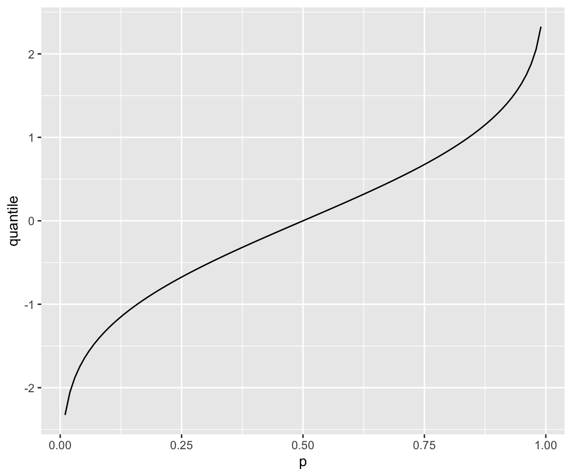
Next, you can take a step further to visualize three different normal distributions in the same plot, \(N(0,1)\), \(N(1,4)\), and \(N(-1, 0.25)\). You can use the same vector x and compute the three pdfs on each element of x. geom_line() is still used with the variable dist mapped to the color aesthetic.
x <- seq(from = -5, to = 5, by = 0.05)
norm_dat_1 <- data.frame(dist = "N(0,1)", x = x, pdf = dnorm(x))
norm_dat_2 <- data.frame(dist = "N(1,4)", x = x, pdf = dnorm(x, mean = 1, sd = 2))
norm_dat_3 <- data.frame(dist = "N(-1, 0.25)", x = x, pdf = dnorm(x, mean = -1, sd = 0.5))
norm_dat <- rbind(norm_dat_1, norm_dat_2, norm_dat_3)
ggplot(norm_dat) +
  geom_line(aes(x = x, y = pdf, color = dist))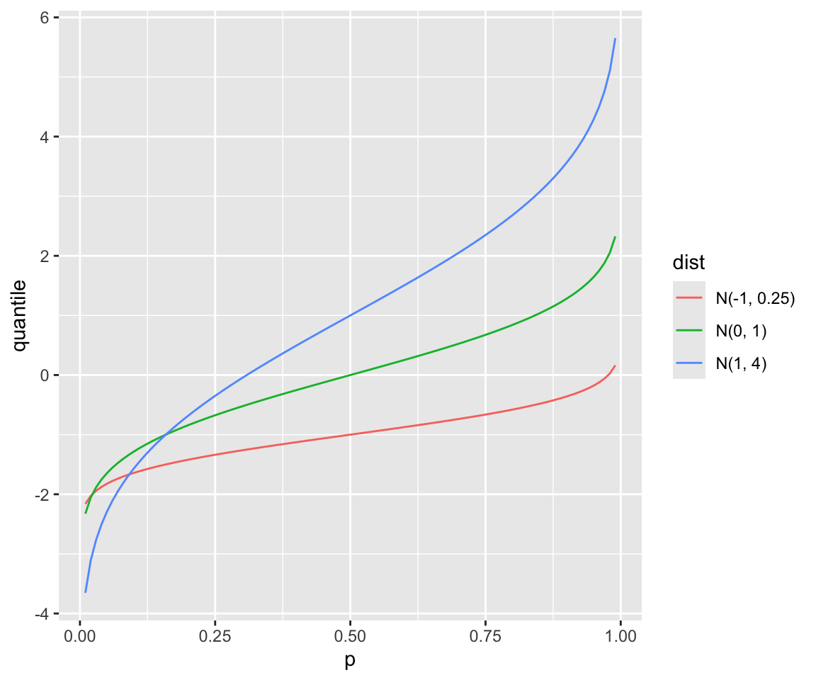
11.1.2 Cumulative Distribution Function (CDF)
In addition to pdf, you can compute the cumulative distribution function (CDF) of the normal distribution using the function pnorm(q, mean, sd). Generally speaking, the CDF of a random variable \(X\) is defined as
\[F(x) = P(X\leq x).\] Similar to dnorm(), pnorm() also has two optional arguments, mean and sd, which represent the mean and standard deviation of the normal distribution, respectively. If you don’t specify these two arguments, pnorm() will compute the CDF of \(N(0,1)\).
You can also use pnorm() to visualize the CDF of the standard normal distribution.
q <- seq(from = -5, to = 5, by = 0.1)
norm_dat <- data.frame(q = q, cdf = pnorm(q))
ggplot(norm_dat) + geom_line(aes(x = q, y = cdf))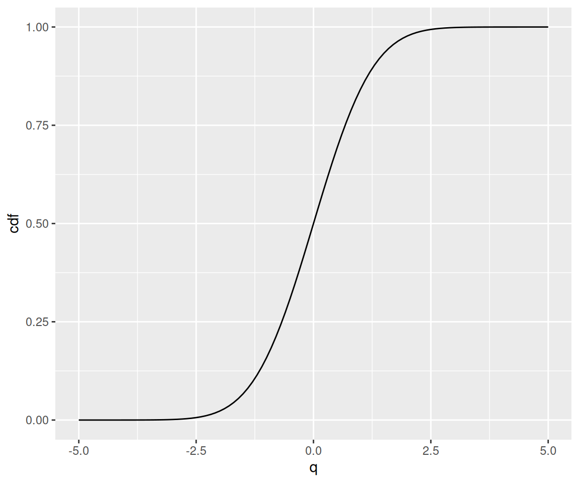
Similarly, you can visualize the CDFs of \(N(0,1)\), \(N(1,4)\), and \(N(-1, 0.25)\).
x <- seq(from = -5, to = 5, by = 0.05)
norm_dat_1 <- data.frame(dist = "N(0,1)", x = x, cdf = pnorm(x))
norm_dat_2 <- data.frame(dist = "N(1,4)", x = x, cdf = pnorm(x, mean = 1, sd = 2))
norm_dat_3 <- data.frame(dist = "N(-1, 0.25)", x = x, cdf = pnorm(x, mean = -1, sd = 0.5))
norm_dat <- rbind(norm_dat_1, norm_dat_2, norm_dat_3)
ggplot(norm_dat) +
  geom_line(aes(x = x, y = cdf, color = dist))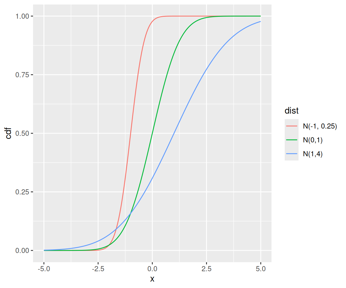
11.1.3 The Empirical Rule (68-95-99.7)
A key property of the normal distribution is the Empirical Rule. It states that for any normal distribution:
- Approximately 68% of the data falls within 1 standard deviation of the mean.
- Approximately 95% of the data falls within 2 standard deviations of the mean.
- Approximately 99.7% of the data falls within 3 standard deviations of the mean.
We can verify this with pnorm(). For a standard normal distribution N(0,1):
# Probability within 1 SD of the mean
prob_1_sd <- pnorm(1) - pnorm(-1)
# Probability within 2 SD of the mean
prob_2_sd <- pnorm(2) - pnorm(-2)
# Probability within 3 SD of the mean
prob_3_sd <- pnorm(3) - pnorm(-3)
cat(sprintf("%% within 1 SD: %.3f\n%% within 2 SD: %.3f\n%% within 3 SD: %.3f\n",
            prob_1_sd, prob_2_sd, prob_3_sd))
#> % within 1 SD: 0.683
#> % within 2 SD: 0.954
#> % within 3 SD: 0.997
11.1.4 Quantile Function
The third useful function related to distributions is the quantile function. It answers the question: “At what value \(x\) is the probability of being less than or equal to it equal to a given probability \(p\)?”
You can compute the quantile of the normal distribution using qnorm(p, mean, sd). The quantile function is the inverse function of the cdf. In particular, the \(p\) quantile returns the value \(x\) such that
\[F(x) = P(X\leq x) = p\]
Let’s verify qnorm() is indeed the inverse function of pnorm() using the following example.
When \(p=0.5\), qnorm() gives us the median of the normal distribution.
Let’s see a few examples for computing the quantiles.
You can also visualize the shape of the quantile function.
p <- seq(from =  0.01, to = 0.99, by = 0.01)
norm_dat <- data.frame(p = p, quantile = qnorm(p))
ggplot(norm_dat) + geom_line(aes(x = p, y = quantile))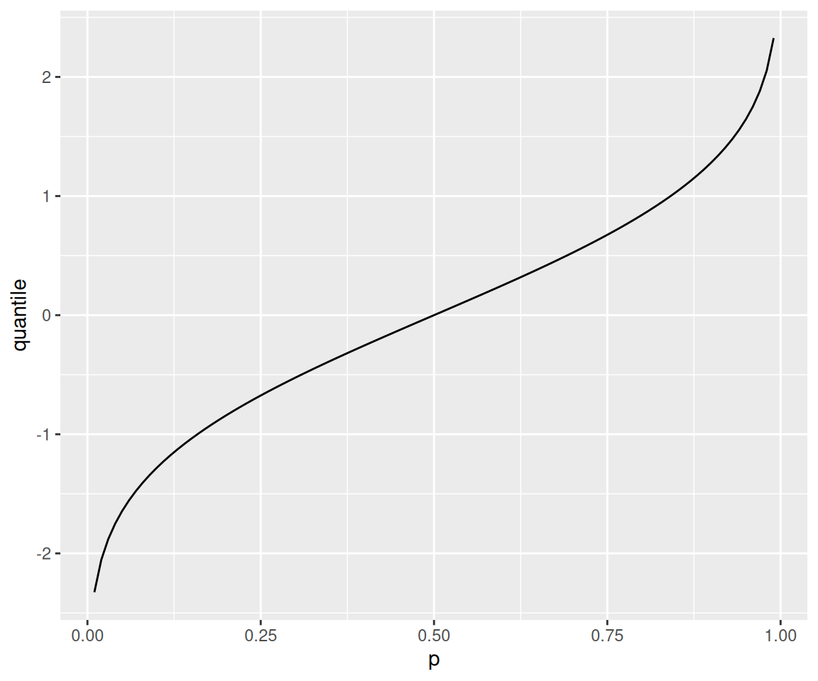
Similarly, you can visualize the quantile files of \(N(0,1)\), \(N(1,4)\), and \(N(-1, 0.25)\).
p <- seq(from =  0.01, to = 0.99, by = 0.01)
norm_dat_1 <- data.frame(dist = "N(0, 1)", p = p, quantile = qnorm(p))
norm_dat_2 <- data.frame(dist = "N(1, 4)", p = p, quantile = qnorm(p, 1, 2))
norm_dat_3 <- data.frame(dist = "N(-1, 0.25)", p = p, quantile = qnorm(p, -1, 0.5))

norm_dat <- rbind(norm_dat_1, norm_dat_2, norm_dat_3)
ggplot(norm_dat) +
  geom_line(aes(x = p, y = quantile, color = dist))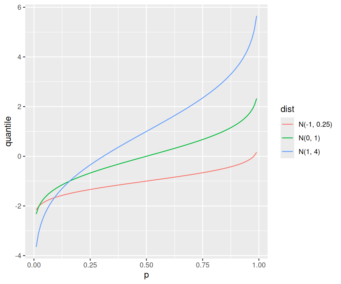
11.1.5 Random Number Generator
Lastly, to generate random numbers from normal distributions, you can use the function rnorm(n, mean, sd) , with the argument n represents the number of random numbers to generate, the arguments mean and sd are the mean and standard deviation of the normal distribution you would like to generate from, respectively. Again, if you only supply the argument n, you will be generating random numbers from \(N(0,1)\).
rnorm(3, mean = 0, sd = 1) #generate 3 random numbers from N(0, 1)
#> [1]  0.9222256 -0.6182918  3.3075975
rnorm(3) #generate another 3 random numbers from N(0,1)
#> [1]  1.2004104 -0.2217104 -0.7454108
Since you are generating random numbers, the results may be different each time. In many applications, however, you may want to make the results reproducible. To do this, you can set random seed using the function set.seed() before generating the random numbers. Let’s see the following example.
Now, let’s run it one more time.
You can see that the exact 3 numbers are reproduced since you are using the same random seed 0. You can run these two lines of code on any machine and will get the exact same three random numbers.
Note that the code that involves randomness needs to be identical to reproduce the results. If you change the arguments in rnorm(), you will get totally different results. See the following example.
By setting a different random seed, you will see different results as the following example.
Lastly, let’s do a simple statistical exercise by checking the closeness of the sample mean and sample standard deviation to their population counterparts.
11.1.6 Exercises
- Compute the PDF of a normal distribution with mean \(\mu=1\) and standard deviation \(\sigma=2\) at locations \(x = -2, 0, 2\). Verify that the output agrees with the formula.
- Plot the PDF of a normal distribution with mean \(\mu=3\) and standard deviation \(\sigma=2\) over the range \(x \in [-4, 4]\).
- Compute the CDF for of a normal distribution with mean \(\mu=1\) and standard deviation \(\sigma=2\) at locations \(q = -1, 0, 1\).
- Plot the CDF of a normal distribution with mean \(\mu=3\) and standard deviation \(\sigma=2\) over the range \(x \in [-4, 4]\).
- Compute the 25th, 50th, and 75th percentiles for a normal distribution with \(\mu = 2\) and \(\sigma = 3\).
- Plot the quantile function for \(p \in [0.1, 0.8]\) for a normal distribution with \(\mu = 2\) and \(\sigma = 3\).
- Generate 1000 random numbers from a standard normal distribution with \(\mu = 0\) and \(\sigma = 1\). Plot the histogram.
- Visualize the histogram in Q7 with the PDF of the standard normal distribution on the same plot, and discuss.
