13.2 Text Formatting in R Markdown

You’ve learned about the powerful YAML header and the utility of R Code Chunks in Section 13.1. Now, your journey continues into the art of text formatting. A well-formatted report is not just professional; it’s a powerful tool to guide your reader through your data story.

R Markdown uses Pandoc’s Markdown, a simple yet powerful syntax for creating beautifully formatted documents. Think of the text in your .Rmd file as your raw materials (marked-up text), and the knitted document as your polished creation (formatted text).

Let’s explore the tools at your disposal.

13.2.1 Headers: Your Document’s Signposts

Use different numbers of hash symbols (#) to create up to six levels of headers. More # symbols mean a lower-level header.

# Level 1: The Chapter Title
## Level 2: A Major Section
### Level 3: A Subsection
#### Level 4: A Sub-subsection
##### Level 5: A Sub-sub-subsection
###### Level 6: A Sub-sub-sub-subsection

Pro-Tip: Set number_sections: true in the YAML header to automatically number your sections.

13.2.2 Emphasis: Making Your Point

Markdown allows you to emphasize text in various ways. Here are some common styles:

Style	Syntax	Example
Italics	`text` or `_text_`	For emphasis or scientific names
Bold	`text` or `__text__`	To show strong importance
~~Strikethrough~~	`~~text~~`	~~This idea was later disproven.~~
`Code Font`	`text`	Use for `function_names()` or `variables`.

13.2.3 Inline Code: Displaying and Evaluating

You can include code within your sentences in two ways:

To display code as text: Wrap it in single backticks. For example, 1 + 1 renders as 1 + 1.
To evaluate code and show its output: Use inline R code with `r `. For example, `r 1 + 1` evaluates to 2 in the output.

Heads‑up: Never wrap code inside a code chunk with back‑ticks: knitr() will treat them as unmatched delimiters and throw an error when you knit.

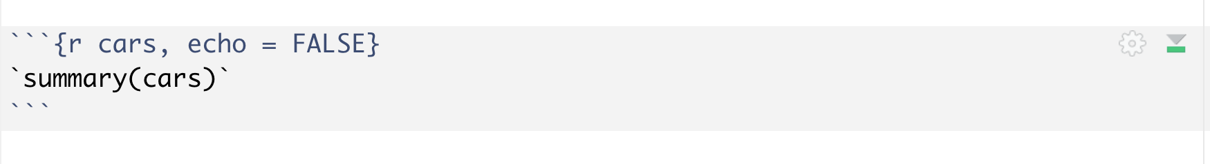
Figure 13.13: Incorrect back-ticks in a code chunck

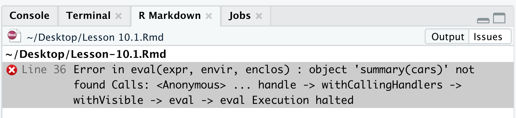
Figure 13.14: The error message

13.2.4 Lists: Ordered and Unordered

Use lists to organize information and break down complex topics.

Unordered Lists: Start each line with *, +, or -.
Ordered Lists: Start each line with a number. R Markdown will automatically sequence them correctly, even if you use 1. for every item.
Nested Lists: Indent items to create sub-lists. You can mix and match ordered and unordered lists.

Here is an example of a mixed list:

1.  First, collect the data.
2.  Second, clean the data.
    * Check for missing values (`NA`).
    * Ensure correct data types.
3.  Finally, analyze the data.

First, collect the data.
Second, clean the data.
- Check for missing values (NA).
- Ensure correct data types.
Finally, analyze the data.

13.2.5 Hyperlinks: Connecting to the World

Guide your readers to external resources with hyperlinks. The format is [Text to display](URL).

I have learned R from the book [r02pro](https://r02pro.github.io/).

This will create a clickable link in the output document that says

I have learned R from the book r02pro.

13.2.6 Blockquotes: Highlighting Wisdom

Use the > character to create a blockquote. This is perfect for quoting sources or emphasizing a key insight.

> "The best thing about being a statistician is that you get to play in everyone's backyard." - John Tukey

This will generate

“The best thing about being a statistician is that you get to play in everyone’s backyard.” - John Tukey

13.2.7 Footnotes: Adding Extra Details

Add non-essential details or citations using footnotes. Use [^1] for the marker and define it anywhere in your document. A more convenient inline method is ^[Your footnote text here.].

This is a statement with a footnote.[^1]

[^1]: This is the footnote text that provides additional information.

This is a statement with a footnote.¹

13.2.8 The Language of the Universe: Writing Mathematics

R Markdown allows you to write beautiful mathematics using LaTeX syntax.

13.2.8.1 Inline Equations

For small formulas that fit within a line of text, wrap your LaTeX code in single dollar signs ($).

**Fun Fact:** Did you know that Euler's Identity, 
$e^{i\pi} + 1 = 0$, connects five of the most fundamental constants in mathematics?

Fun Fact: Did you know that Euler’s Identity, $e^{i\pi} + 1 = 0$, connects five of the most fundamental constants in mathematics?

13.2.8.2 Displayed Equations

For larger equations that deserve their own line, wrap them in double dollar signs ($$).

*Statistical Insight:* The probability density function of the normal distribution $N(\mu, \sigma^2)$, a cornerstone of statistics, is given by:
$$ f(x) = \frac{1}{\sqrt{2\pi\sigma^2}} e^{-\frac{(x-\mu)^2}{2\sigma^2}} $$

Statistical Insight: The probability density function of the normal distribution $N(\mu, \sigma^2)$, a cornerstone of statistics, is given by: \[ f(x) = \frac{1}{\sqrt{2\pi\sigma^2}} e^{-\frac{(x-\mu)^2}{2\sigma^2}} \]

13.2.9 Tables: From Simple to Stunning

While you can write tables by hand in Markdown, it’s far more powerful to generate them with R. The knitr::kable() function is your starting point.

For a simple table, you can create a data frame in R:

df <- data.frame(Statistic = c("Mean", "Median", "Standard Deviation"), R_Function = c("`mean()`",
    "`median()`", "`sd()`"), Description = c("The average value", "The middle value",
    "A measure of spread"))
knitr::kable(df, caption = "Common Descriptive Statistics in R")

Table 13.1: Common Descriptive Statistics in R
Statistic	R_Function	Description
Mean	`mean()`	The average value
Median	`median()`	The middle value
Standard Deviation	`sd()`	A measure of spread

Power-Up with kableExtra: For truly publication-quality tables, the kableExtra package is a must-have. It allows for advanced styling.

# You may need to run this once in your Console: install.packages('kableExtra')
library(kableExtra)

# Let's show some fun facts about planets
planets_df <- data.frame(Planet = c("Mercury", "Earth", "Mars", "Jupiter"), Type = c("Terrestrial",
    "Terrestrial", "Terrestrial", "Gas Giant"), Moons = c(0, 1, 2, 95), `Gravity (m/s^2)` = c(3.7,
    9.8, 3.7, 24.8), check.names = FALSE)

kable(planets_df, caption = "Fun Facts About Our Solar System Neighbors") %>%
    kable_styling(bootstrap_options = c("striped", "hover", "condensed"), full_width = FALSE) %>%
    column_spec(2, bold = TRUE) %>%
    add_header_above(c(` ` = 1, Classification = 1, Satellites = 2))

Table 13.2: Fun Facts About Our Solar System Neighbors
	Classification	Satellites
Planet	Type	Moons	Gravity (m/s^2)
Mercury	Terrestrial	0	3.7
Earth	Terrestrial	1	9.8
Mars	Terrestrial	2	3.7
Jupiter	Gas Giant	95	24.8

This will create a table with a header row and some styling applied.

13.2.10 Insert citations and manage bibliographies in R Markdown

R Markdown provides us the capability to add bibliography and manage citations with ease, similar to writing a LaTex document. To add citations, you first need to add the bibliography filed in the YAML head. If your references are in the file “references.bib”, you can set the bibliography file as follows.

---
output: html_document
bibliography: references.bib  
---

The .bib file is a plain-text file that consists of bibliography entries like the following:

@book{r02pro,
  title = {R Programming: From Zero to Pro},
  author = {Yang Feng},
  organization = {New York University},
  address = {New York, NY},
  year = {2024},
  url = {https://r02pro.github.io/},
}

Then, each bibtex items can be cited directly within the documentation using the syntax @key, where key is the citation key in the first line of the entry, e.g., @r02pro will show as Feng (2024) in the document. To put citations in parentheses, use [@key]. To cite more than one items, separate the keys by semicolons, e.g., [@key-a; @key-b; @key-c]. To suppress the author name, you can add a minus sign before @, e.g., [-@r02pro] will generate (2024).

To learn more about citations and bibliography in R Markdown, you can read the excellent book by Xie, Dervieux, and Riederer (2020)..

13.2.11 Your Turn: A Mini-Challenge

Time to get your hands dirty! Create a new .Rmd file and try to build the following mini-report. This is the best way to solidify your new skills.

Create a Level 1 Header: “My Favorite Mathematical Constant”
Write a sentence in bold explaining what your favorite constant is (e.g., My favorite constant is $\pi$).
Add a blockquote with a fun fact about it.
Create an ordered list with at least two reasons why you like it.
Include an inline R calculation. For example: “A circle with a radius of 5 units has a circumference of `r 2 * pi * 5` units.”
Add a footnote with a link to a Wikipedia article about your chosen constant.

Good luck, and happy formatting!

An example .Rmd file is below for your reference.

---
title: "Mini-Challenge Solution: My Favorite Mathematical Constant"
output: html_document
---

# My Favorite Mathematical Constant

**My favorite constant is  $e$**

> Euler's number, $e$, is approximately 2.71828 and is the base of the natural logarithm. It appears everywhere in growth processes, probability, and calculus!

Here are a few reasons why I like $e$:

1. It describes continuous growth and exponential change perfectly.
2. It has deep connections to calculus, particularly in limits and derivatives.

For example, if something grows continuously at a rate of 100%, after 1 unit of time it grows to:

`r exp(1)` units.

You can learn more about $e$ on its [Wikipedia page](https://en.wikipedia.org/wiki/E_(mathematical_constant)).[^1]

[^1]: Wikipedia article: https://en.wikipedia.org/wiki/E_(mathematical_constant)

References

Feng, Yang. 2024. R Programming: From Zero to Pro. New York, NY: New York University. https://r02pro.github.io/.

Xie, Yihui, Christophe Dervieux, and Emily Riederer. 2020. R Markdown Cookbook. Chapman; Hall/CRC.

This is the footnote text that provides additional information.↩︎